| ID |
Date |
Author |
Subject |
|
8
|
Fri Feb 22 17:09:28 2019 |
Suren Gourapura | Updates that need to be added to the manual | We are redesigning the way we simulate antennas in our loop. To do this, we changed our simulationPEC macro skeletons and our output skeleton.
To make this easier, we changed the way we name the files, from i.uan where i is the simulation number, to i_j.uan where i is the antenna and j is the frequency.
We also rewrote XFintoARA.py so it's clean. Note that before there were comments from a previous author claiming it was VERY questionably written. This has now been cleaned up. We also changed the bash script relevant to the above changes.
This change needs to be added to the manual, and until we update this update, we have not done it.
|
|
218
|
Thu May 11 15:57:08 2023 |
Ryan Debolt, Byran Reynolds | AREA Updates | Here is some backlogged information as well as recent updates to our progress on AREA and its optimizations:
4/13/2023
We concluded our initial test of the AREA optimization loop. While analyzing our results, we noticed that most of our runs never reached our benchmarks for performance (chi-squared scores of .25 and .1) and that those that did contain abnormally high amounts of mutation. From previous runs using the GA for the GENETIS loop, we find that mutation and immigration (Note: AREA does not use immigration) usually play a smaller role in overall growth and are simply there to promote diversity. Crossover on the other hand is what handles the bulk of the growth done by the GA. Given our results ran counter to that, we decided to look further into the matter.
Upon looking at the fitness score files, we could see that mutation-created individuals did not perform well in the best run types, but the crossover ones did contain the bulk of good scores. This lines up with expectations. However, closer inspection revealed that these crossover-derived individuals had extremely similar fitness scores, which could indicate elitism in selection methods leading to a lack of diversity in solutions. We then looked at a run that used only crossover with one selection type (roulette), and found every individual to have identical (and poor) scores that were the same up to around the 4th decimal place. This is a strong case that the selection methods used are too elitist to grow a population properly.
We dove into the AREA GA to take a look at the functions doing the selection methods, and discovered several issues potentially causing excess elitism in the GA. It seems that the roulette selection does not behave the way we have used in our other GAs. There appears to be no weighting of individuals; rather, a threshold fitness score is collected and only individuals with a fitness score above the threshold are selected. This causes elitism, as only the most fit individuals are likely to pass this threshold. Tournament was found to be similarly troubled, with a bracket size of ⅓ of the population. This is again very elitist, as it is very large, making it very likely that only the best individuals will be selected. Before we try to further optimize the AREA GA, these selection methods should be addressed and fixed.
For roulette, we propose implementing a similar weighting scheme for individuals as is used in the PAEA GAs that gives preference to the most fit individuals, but still allows others to be selected to encourage diversity of solutions.
For crossover, we propose decreasing the bracket size. This would allow a more diverse range of individuals to be selected through “winning” smaller brackets that would have a lower probability of including top performing individuals.
4/20/23
We (Bryan and Ryan) met to work on improving the selection method functions in the AREA algorithm.
For roulette selection, we added weighting by fitness score, as is done in the other GENETIS GAs, in an effort to prevent it from disproportionately selecting the most fit individuals only to become parents. As a first test, we ran an abbreviated version of the test-loop code, printing the fitness scores of the parents selected by the roulette method. The fix appears to have passed this initial test, as the fitness scores showed more variety and in the case of roulette crossover two unique parents seemed to be selected.
For tournament selection, the only change necessary appeared to be decreasing the bracket size of the tournament(s), which in turn encourages other individuals besides the most fit to be selected as parents, therefore increasing diversity of solutions. We ran out of time to test this change fully, so we will pick up here in our next meeting.
Looking further ahead, we will plan to work on refactoring the AREA algorithm to use the same functions as the other GENETIS GAs wherever possible. In the meantime, this working version can still be used for feature development so that progress is not halted.
5/11/2023
Upon looking at the results of the recent optimizations, our best runs are still taking over 40 generations to reach an optimized score. Given the speed of AraSim, this is still too slow to be considered optimal. Comparing this test loop run to the ones run on by the broader GENETIS GA, our best runs for the AREA GA are worse than the worst runs from those optimizations. As such, we have decided to pause optimizing the AREA GA in favor of adding it to the broader GENETIS one. As of today, we have finished a rough version of the generating function necessary to create new individuals. We have also started progress on the constraining functions and scaling functions that will be necessary to generate the spherical harmonics used to find the gain and phase. Once these functions are complete, we should be able to transplant this GA back into our test loop for AREA and resume optimizations.
|
|
220
|
Thu May 25 15:36:54 2023 |
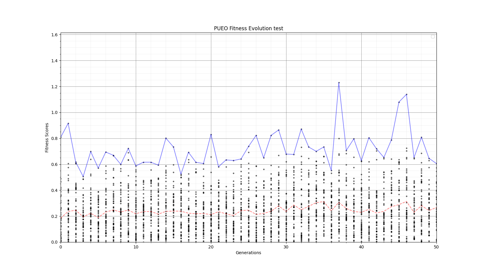
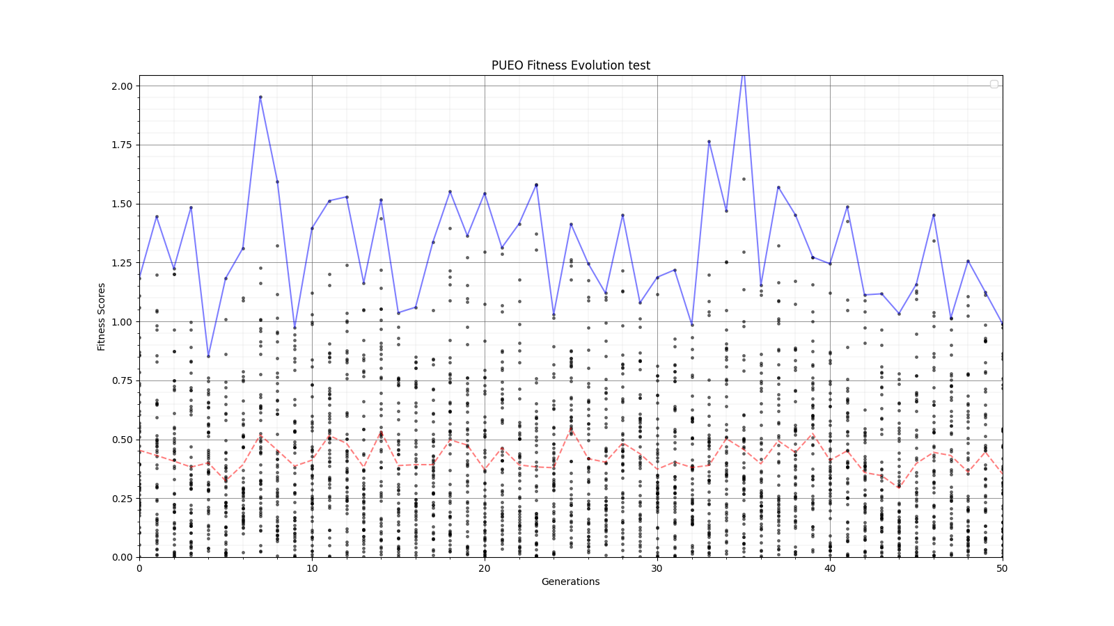
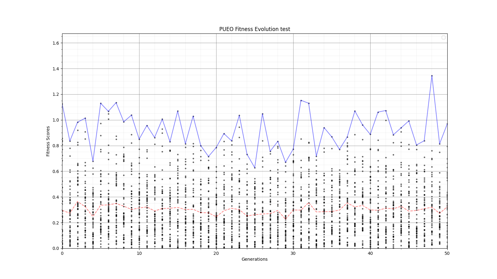
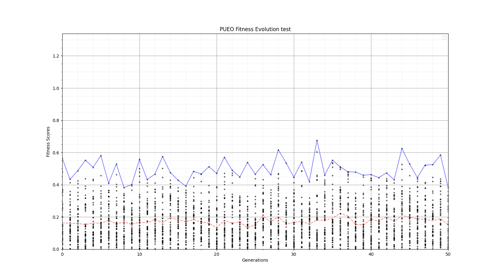
Ryan Debolt, Byran Reynolds | preliminary error tests (PUEO) | Here are some preliminary results from testing the effect of error on growth in the GA. For this test, we start with a simulated error of 0.5 because our true fitness score is bounded between 0.0 and 1.0. From here, we simulate doubling the number of neutrinos by reducing the error by root(2), then root(4), and observed the growth on the fitness scores plots. We did these three tests with both 50 and 100 individuals (plots starting with 30 use 50 and starting with 60 use 100). Looking at the plots, we can see that the only plot that shows growth is 100 individuals with halved error (corresponding to 4 times the number of neutrinos). In fact, it took going to root(25) (corresponding to 25 times the number of neutrinos) to observe comparable growth with 50 individuals. This leads us to believe we likely need to increase both neutrinos and individuals to see meaningful growth in our GA. Further tests are required to see how consistent these results are. Another test, though unrealistic, we ran 1000 individuals with the root(25), this test was optimized in around 10 generations, this could be seen as a maximum performance standard. |
| Attachment 1: 30_10_10_0_48_25_6_2_half_error_fitness.png
|  |
| Attachment 2: 30_10_10_0_48_25_6_2_high_error_fitness.png
|  |
| Attachment 3: 30_10_10_0_48_25_6_2_root2_error_fitness.png
|  |
| Attachment 4: 30_10_10_0_48_25_6_2_root8_error_fitness.png
|  |
| Attachment 5: 30_10_10_0_48_25_6_2_root25_error_fitness.png
| 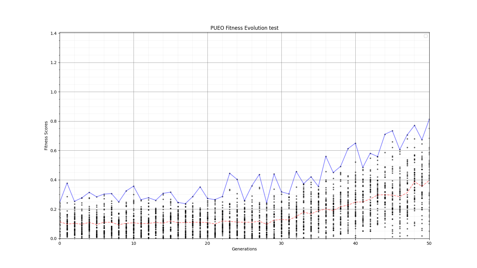 |
| Attachment 6: 60_20_20_0_96_25_6_1_half_error_fitness.png
| 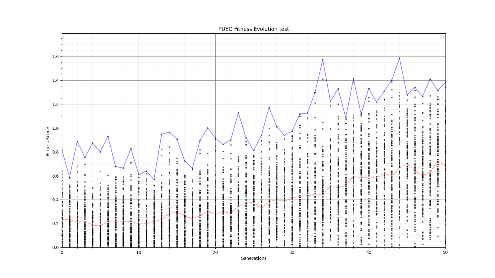 |
| Attachment 7: 60_20_20_0_96_25_6_1_high_error_fitness.png
| 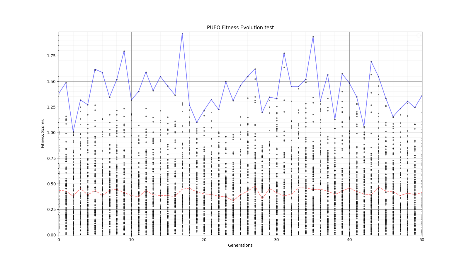 |
| Attachment 8: 60_20_20_0_96_25_6_1_root2_error_fitness.png
| 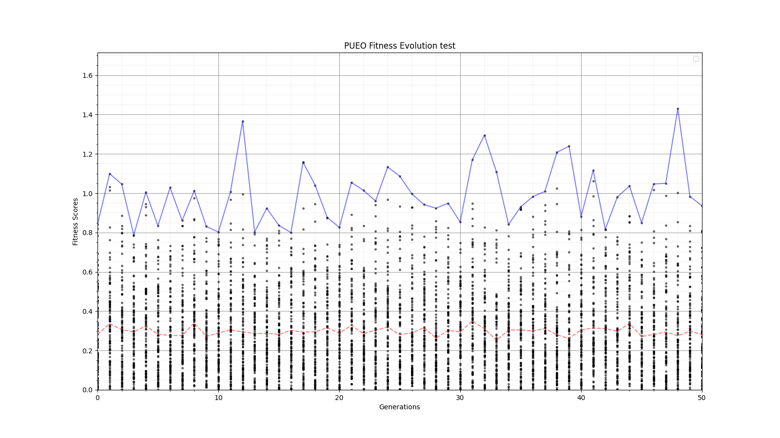 |
|
Draft
|
Fri Aug 21 15:19:10 2020 |
Ryan Debolt | Friday Updates |
| Name |
Update |
Plans for next week |
| Alex M |
|
|
| Alex P |
|
|
| Eliot |
|
|
| Leo |
|
|
| Evelyn |
|
|
| Ryan |
This week I completed work on a set of graphs that shows many instances of of a run type on a graph to show the spread that runs give. I am still working on finishing up the plots that show averages of roulette to tournament for each sigma but the should be finished soon. |
Finish the aforementioned plot. |
| Ben |
|
|
| Ethan |
Ben and I spent the week working on two seperate python scripts, one to plot the fitness scores of each child in each generation, and another to replace dummy Veff scores with Veff scores found in another file. We also updated the documentation on OverLeaf. |
On monday we will continue to keep updating the documentation as well as continueing to imporve AREA. |
|
|
120
|
Mon Nov 23 18:02:40 2020 |
Ryan Debolt | Monday Updates |
| Alex M |
Kept working with Amy, Alex P, Julie, and Ben on the AraSim fix. We fixed our issue from last week but have a new one in stage 2. It looks like the issue has to do with resetting the values for V_forfft right before stage 2 (around line 963). Check here for the current version of Report.cc: /users/PAS0654/pattonalexo/EFieldProject/11_23_20 |
| Ryan |
Fixed the issue with the segmentation faults in the GA (simple fix one line changed) and worked with Kai to start creating a spreadsheet of results. Results seem to suggest that 2 tournament to 8 roulette seems to be the ideal selection ratio and the initial test seem to suggest a small amount of reproduction is ideal but more testing is needed to confirm this. |
| |
|
| |
|
| |
|
| |
|
| |
|
|
|
142
|
Fri Feb 4 16:50:09 2022 |
Ryan Debolt | Loop Run |
- Run Type
- Run Date
- Run Name
- Why are we doing this run?
- To test rank selection in main loop
- What is different about this run from the last?
- Rank Slection is being used.
- Parents.csv introduced.
- Elite is being turned off.
- Symmetric, asymmetric, linear, nonlinear (what order):
- Number of individuals (NPOP):
- Number of neutrinos thrown in AraSim (NNT):
- Operatiors used (% of each):
- 06% Reproduction
- 72% Crossver
- 22% Immigration
- 1% M_rate (unused)
- 5% sigma (unused)
- Selection methods used (% of each):
- 0% Elite
- 0% Reproduction
- 10% Tournament
- 90% Rank
- Are we using the database?
Directory: /fs/ess/PAS1960/BiconeEvolutionOSC/BiconeEvolution/current_antenna_evo_build/XF_Loop/Evolutionary_Loop/Run_Outputs/2022_02_04_Rank |
| Attachment 1: run_details.txt
|
####### VARIABLES: LINES TO CHECK OVER WHEN STARTING A NEW RUN ###############################################################################################
RunName='2022_02_04_Rank'	## This is the name of the run. You need to make a unique name each time you run.
TotalGens=100			## number of generations (after initial) to run through
NPOP=50				## number of individuals per generation; please keep this value below 99
Seeds=10			## This is how many AraSim jobs will run for each individual## the number frequencies being iterated over in XF (Currectly only affects the output.xmacro loop)
FREQ=60				## the number frequencies being iterated over in XF (Currectly only affects the output.xmacro loop)
NNT=30000			## Number of Neutrinos Thrown in AraSim
exp=18				## exponent of the energy for the neutrinos in AraSim
ScaleFactor=1.0			## ScaleFactor used when punishing fitness scores of antennae larger than the drilling holes
GeoFactor=1			## This is the number by which we are scaling DOWN our antennas. This is passed to many files
num_keys=4			## how many XF keys we are letting this run use
database_flag=0			## 0 if not using the database, 1 if using the database
				## These next 3 define the symmetry of the cones.
RADIUS=1			## If 1, radius is asymmetric. If 0, radius is symmetric
LENGTH=1			## If 1, length is asymmetric. If 0, length is symmetric
ANGLE=1				## If 1, angle is asymmetric. If 0, angle is symmetric
CURVED=1			## If 1, evolve curved sides. If 0, sides are straight
A=1				## If 1, A is asymmetric
B=1				## If 1, B is asymmetric
SEPARATION=0    		## If 1, separation evolves. If 0, separation is constant
NSECTIONS=2 			## The number of chromosomes
DEBUG_MODE=0			## 1 for testing (ex: send specific seeds), 0 for real runs
				## These next variables are the values passed to the GA
REPRODUCTION=3			## Number (not fraction!) of individuals formed through reproduction
CROSSOVER=36			## Number (not fraction!) of individuals formed through crossover
MUTATION=1			## Probability of mutation (divided by 100)
SIGMA=5				## Standard deviation for the mutation operation (divided by 100)
ROULETTE=0			## Percent of individuals selected through roulette (divided by 10)
TOURNAMENT=1			## Percent of individuals selected through tournament (divided by 10)
RANK=9				## Percent of individuals selected through rank (divided by 10)
ELITE=0				## Elite function on/off (1/0)

#####################################################################################################################################################
|
|
143
|
Fri Feb 4 17:59:41 2022 |
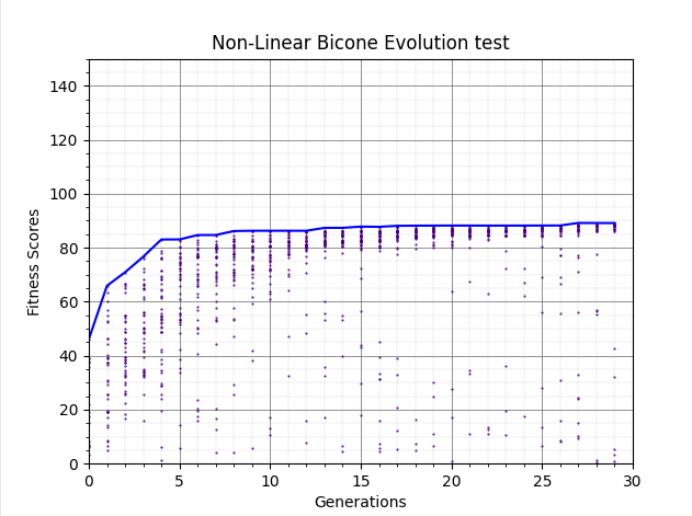
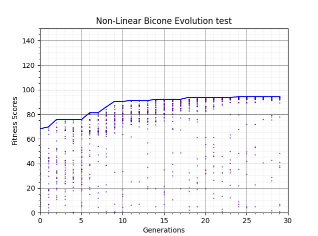
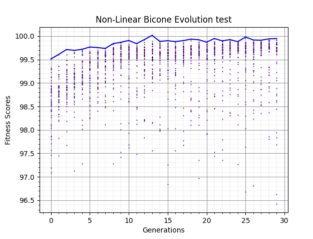
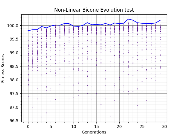
Ryan Debolt | GA Updates | The following plots are ittereations if the test loop that add increasing improvements to the GA.
The first plot shows the GA's behavoir unaltered from our previous runs (80% roulette, 20% tournament elite selection on).
The second plots shows when we use 90% rank selection and 10% tournament, elite selection off.
Plot 3 shows when we add an offset to restrict the values of the fitness function to be more within the range of the main loop.
Plot 4 shows when we add a gaussean mutation function that is applied to crossover individuals (rate and gaussean width chosen by guess).
The following are papers I have looked at while modifing the GA (not nessisaraly recently).
https://pdfs.semanticscholar.org/5733/418cbf21dedc9e5c04351ded4a989f1ff67e.pd
https://www.sciencedirect.com/science/article/abs/pii/0165607493902157
https://www.scientific.net/AMM.340.727
http://citeseerx.ist.psu.edu/viewdoc/download?doi=10.1.1.28.1400&rep=rep1&type=pdf
https://arxiv.org/pdf/2010.04340.pdf
https://d1wqtxts1xzle7.cloudfront.net/30694440/10.1.1.34.9722.pdf?1361979690=&response-content-disposition=inline%3B+filename%3DUsing_genetic_algorithms_with_asexual_tr.pdf&Expires=1612908683&Signature=X93Gsc47AS0xqWf1SPLjG~7sNkoXSOXfnq1GpZ2QaPrYw9x9mWwASStW2IWexo7QBzbkhzcE5tZ~CmQA1MHN-paiNFIx2ed8VNS3IhesMnotKM0mSgUZ37BCleHT9BgGkUUum8mTJBAzCUaECn6RYjm1CZpfwVPC9zwuA~DnXBST4pGlQdna22D--sHwXgX~3U3gDUSxqk8mLI0gtn~Xued3XqsTGuMUKwJ2D9UpD5yp42-3IrH6d5CZREjEfXY2geTopQ-uNkr3eOriDj0UZqSrDw5mczmod3kQrQncgd~G2Kyda4RlIs8VDzQs~BGgszHJhSDAuKDrXr8P--9tVg__&Key-Pair-Id=APKAJLOHF5GGSLRBV4ZA
http://citeseerx.ist.psu.edu/viewdoc/download?doi=10.1.1.438.7389&rep=rep1&type=pdf
https://arxiv.org/pdf/2102.01211.pdf |
| Attachment 1: Original_Params.PNG
|  |
| Attachment 2: Rank_params.PNG
|  |
| Attachment 3: Range_restriction.PNG
|  |
| Attachment 4: Mutation.PNG
|  |
|
145
|
Fri Feb 11 16:09:24 2022 |
Ryan Debolt | Parents.csv | Below is an example of our Parents.csv file written by the GA. This file tracks the parents of the individuals of the current generation. The columns and their contained information are as follows:
Current Gen:
The numbered individual of the current generation.
Parent 1:
The number of the first parent of this individual as read from the previous generation.
Parent 2:
The number of the first parent of this individual as read from the previous generation.
Operator:
The genetic operator that created the individual in that row. |
| Attachment 1: Parents.csv
|
Location of individuals used to make this generation:


Current Gen, Parent 1, Parent 2, Operator
1, 15, NA , Reproduction
2, 22, NA , Reproduction
3, 35, NA , Reproduction
4, 34, 39, Crossover
5, 34, 39, Crossover
6, 35, 29, Crossover
7, 35, 29, Crossover
8, 37, 5, Crossover
9, 37, 5, Crossover
10, 28, 12, Crossover
11, 28, 12, Crossover
12, 5, 22, Crossover
13, 5, 22, Crossover
14, 18, 23, Crossover
15, 18, 23, Crossover
16, 3, 33, Crossover
17, 3, 33, Crossover
18, 28, 14, Crossover
19, 28, 14, Crossover
20, 2, 17, Crossover
21, 2, 17, Crossover
22, 23, 22, Crossover
23, 23, 22, Crossover
24, 13, 15, Crossover
25, 13, 15, Crossover
26, 31, 35, Crossover
27, 31, 35, Crossover
28, 42, 13, Crossover
29, 42, 13, Crossover
30, 17, 6, Crossover
31, 17, 6, Crossover
32, 1, 5, Crossover
33, 1, 5, Crossover
34, 29, 38, Crossover
35, 29, 38, Crossover
36, 19, 10, Crossover
37, 19, 10, Crossover
38, 9, 38, Crossover
39, 9, 38, Crossover
40, NA, NA, Immigration
41, NA, NA, Immigration
42, NA, NA, Immigration
43, NA, NA, Immigration
44, NA, NA, Immigration
45, NA, NA, Immigration
46, NA, NA, Immigration
47, NA, NA, Immigration
48, NA, NA, Immigration
49, NA, NA, Immigration
50, NA, NA, Immigration
|
|
147
|
Thu Feb 24 20:08:46 2022 |
Ryan Debolt | Parents | |
| Attachment 1: Parent_tracking_example.pdf
|
|
150
|
Fri Apr 1 16:35:50 2022 |
Ryan Debolt | Population test. | https://docs.google.com/spreadsheets/d/1vvcmjByKfcns0-tbAjtePB8ZVGsXAKxXCfbMc99weMI/edit?usp=sharing Here is the spreadsheet link for the population test. |
|
155
|
Fri May 20 17:17:32 2022 |
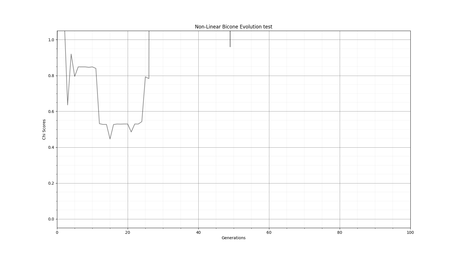
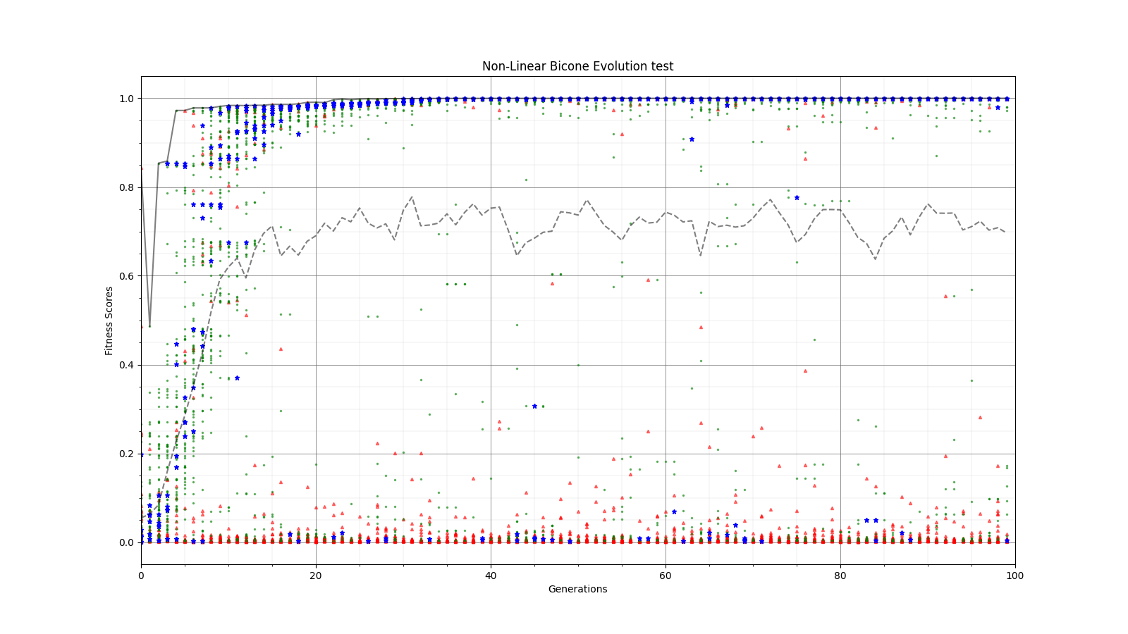
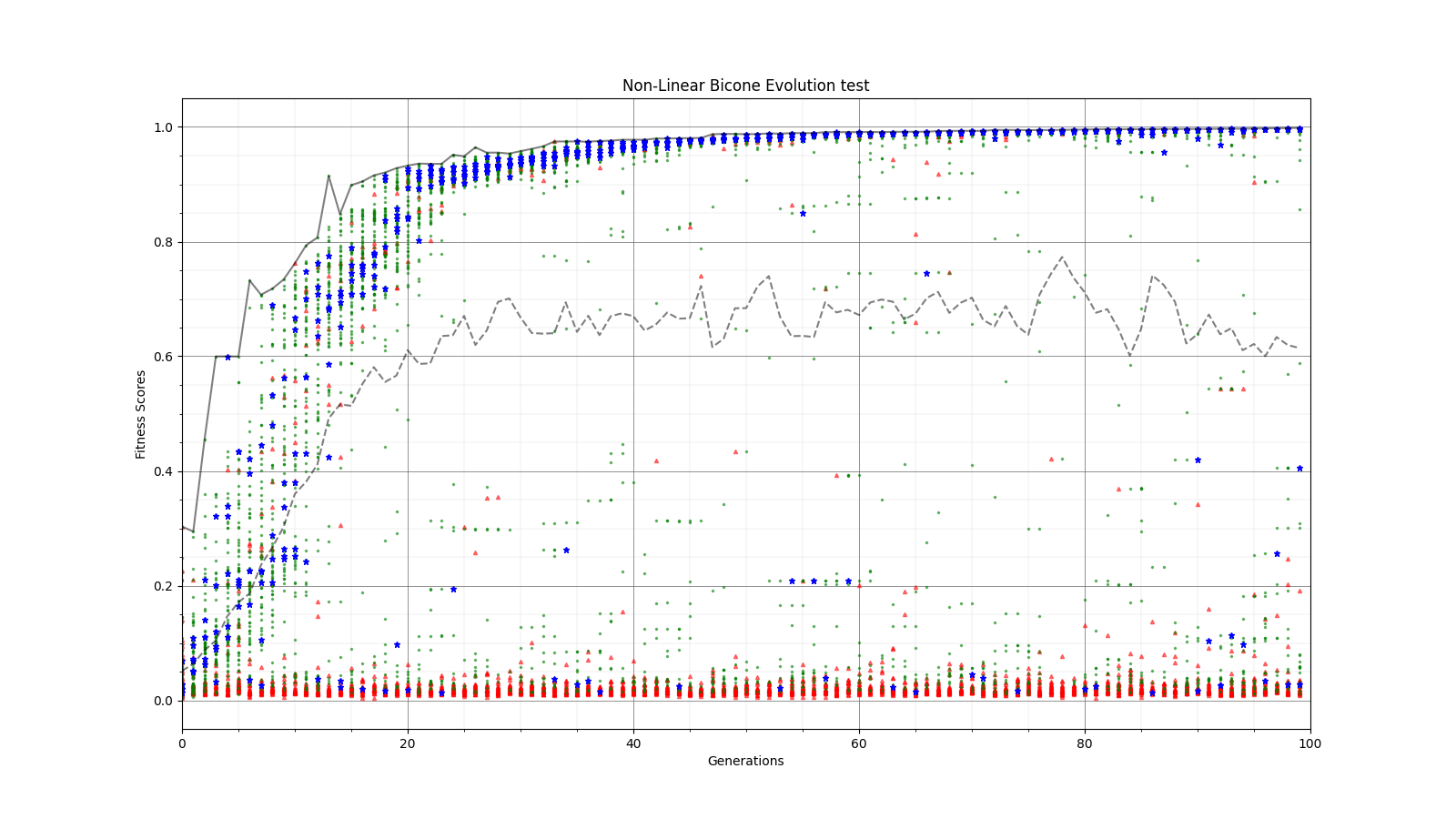
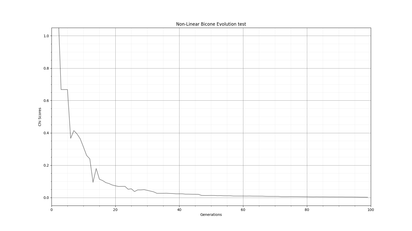
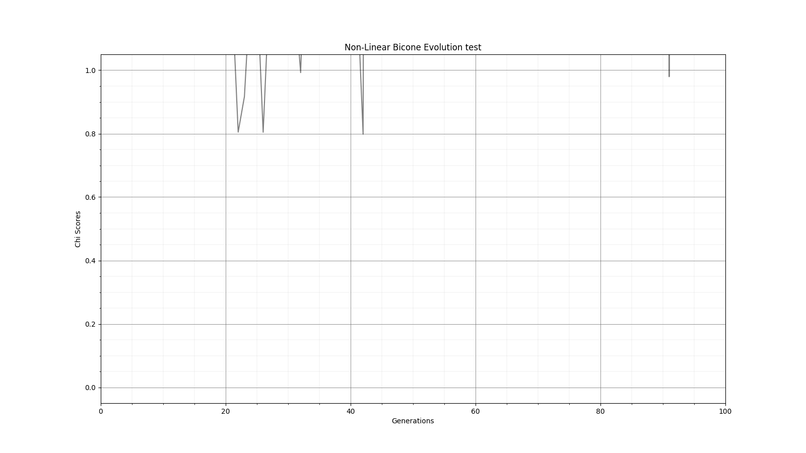
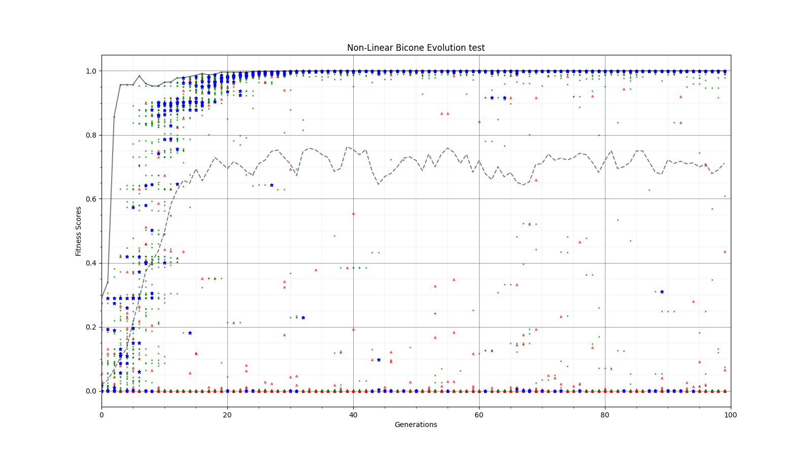
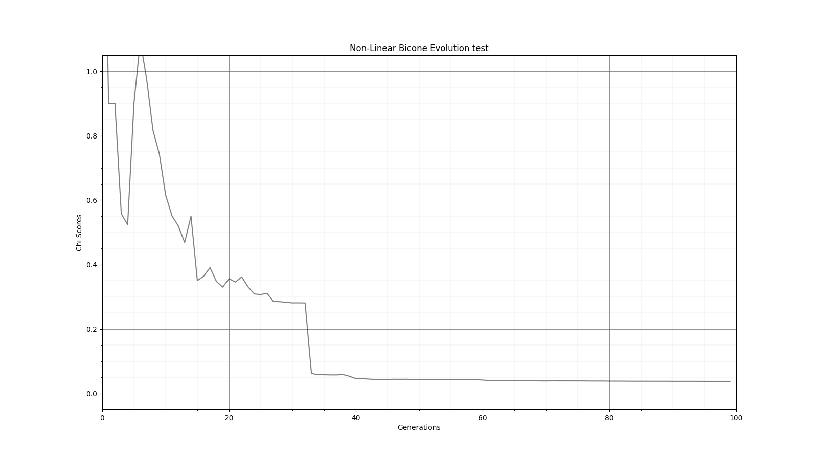
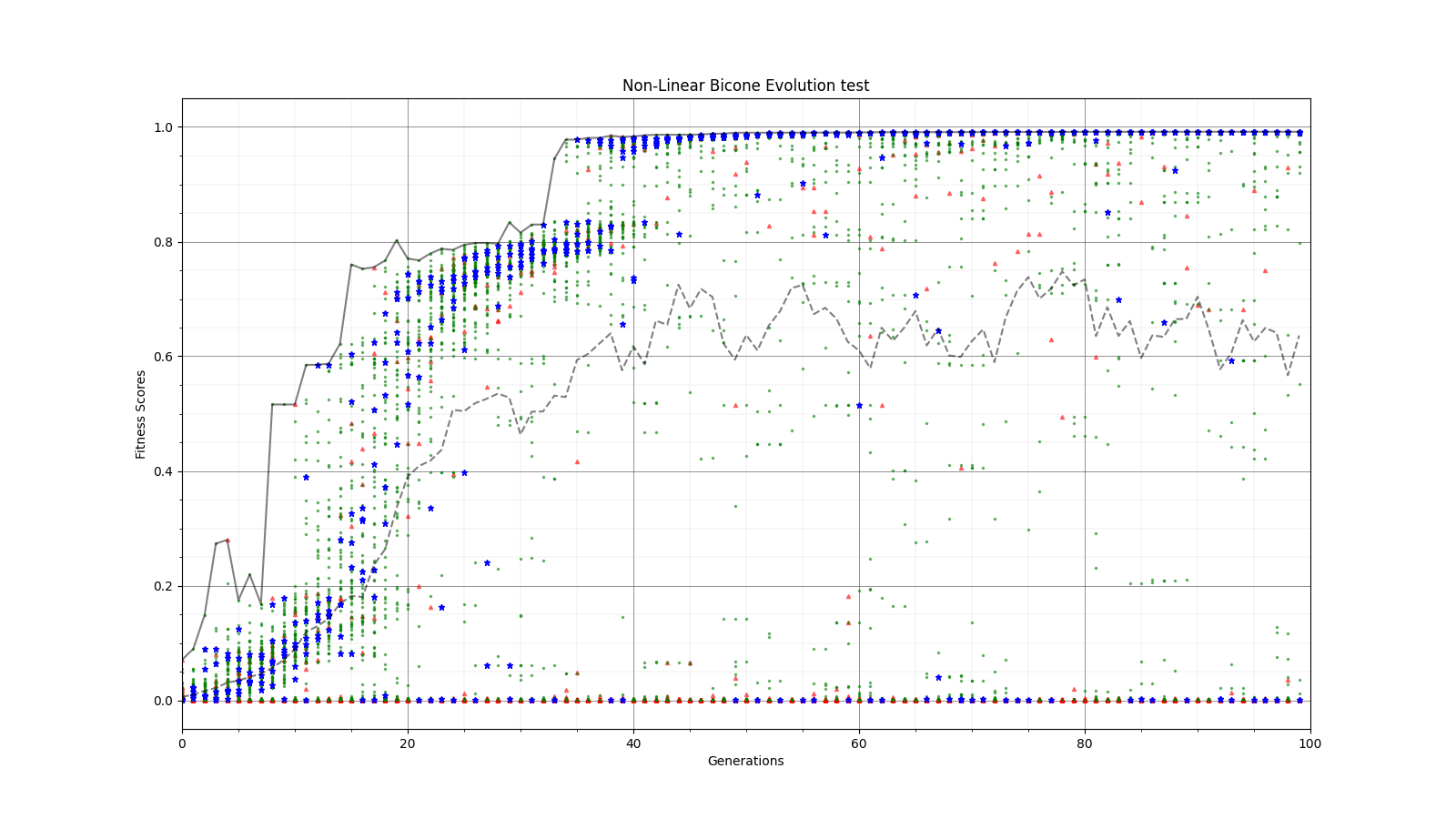
Ryan Debolt | Fitness Functions Test | Bellow lies plots testing different scores and comparing them using a chi^2 score.
The functions used are as follows
Gaussian: e^(-2) (Red)
Inverse: 1/(1+(O-E)^2) (Purple)
Algebraic: 1/(1+(chi^2) )^(3/2)) (Green)
Chi: 1/(1+chi^2) (Blue)
Which are plotted here:

|
| Attachment 1: Alg_Chi.png
|  |
| Attachment 2: Alg_fitness.png
|  |
| Attachment 3: inv_Chi_Fitness.png
|  |
| Attachment 4: Inv_Chi_Chi.png
|  |
| Attachment 5: Gauss_Chi.png
|  |
| Attachment 6: Gauss_Fitness.png
|  |
| Attachment 7: Inv_Chi.png
|  |
| Attachment 8: Inv_Fitness.png
|  |
|
166
|
Tue Jun 21 13:20:41 2022 |
Ryan Debolt | Multigenerational Narrative draft | The story of individual 8 from generation 18. (draft)
Once, there was a curved bicone named individual 8 who was from generation 18. In many ways, it was similar to many other bicones but in fact, this individual was the best bicone that ever lived with a fitness score of 5.22097. It achieved this by having the following parameters; an inner radius of 6.31483, and 3.97024; lengths of 77.6017 and 40.9244; quadratic coefficients of, 0.00260615 and, -0.0103313; and finally, a linear coefficient of -0.197494 and
0.36119. Unfortunately, individual 8’s lineage ended with it as it never met that special someone (crossover) and didn't survive into the next generation (reproduction) despite having a 77.7% of doing at least one of these.
This bicone had a sibling with a fitness Score of 4.65861 and had the following parameters: 6.05614,79.663,-0.000353038,0.0331969 (side 1)
1.92878,37.9849,-0.00213265,0.156724 (side 2).
Unfortunately, this bicone also suffered the same fate as its sibling and failed to leave a lasting mark on this hypothetical world.
These two individuals had parents from generation 17 whose name’s were individuals 39 and individual 8. After having individuals 8 and 9 in generation 18, individuals 39 and 8 from generation had a nasty divorce (possibly leading to 8 and 9’s aversion to marriage) and remarried. In these marriages, they both produced two more children that would be our previous antenna’s step-siblings.
Antenna 8 from gen 17 married antenna 46 to produce antenna 20 with a fitness score of 4.57122, and antenna 21 with a fitness score of 4.71056. Individual 20 shared the same genes for the second set of linear and quadratic coefficients as its more successful step-sibling individual 8. 21 had no similarities to individual 8 but had 4 children in generation 19.
Antenna 39 from gen 17 married antenna 5 to produce antenna 28 with a fitness score of 4.71808 and antenna 29 with a fitness score of 4.90119. Antenna 28 shared had an identical side 1 to individual 8 and also shared the same inner radius and length on the second side, and had 2 children in generation 19. Individual 29 had no similarities to individual 8 but really got around and had 8 children with various partners in generation 19. |
|
Draft
|
Thu Jun 30 13:04:48 2022 |
Ryan Debolt | Multigenerational Narrative draft 2 | This is a multigenerational tracing of our second-best individual's parents and children:
The second-best individual in this evolution was Bicone 22 from generation 40. This individual is, in fact, a fascinating case as we shall see. But to start the story of this individual we will go back to generation 38 in order to demonstrate some of the peculiarities.
In generation 38 there were two bicones of no renown, Bicone 11 and Bicone 17. Bicone 11 was a fairly average individual that was ranked 23rd with a fitness score of 4.72016. Its DNA was {*6.16084, ***79.663, 0.0015434, -0.107765} for side one , and {0.308809, 39.6742, -0.0084247, 0.40629} for side two. One day, by chance it met Bicone 17, another average bicone ranked 24th with a score of 4.71877 and DNA {**2.32499, 79.663, -0.00224948, 0.192602} for side one, and {0.308809, 39.6742, -0.0084247, 0.40629} for side two. These two individuals eventually became the parents of two antennas: Bicone 16 and Bicone 17 of generation 39.
Bicone 16 eventually grew to have been ranked 3rd in fitness score of 4.95323. It’s DNA ended up being a complete balance of its parents sharing side one with Bicone 38.11{2.32499, 79.663, -0.00224948, 0.192602} and side two with bicone 38.17 {0.308809, 39.6742, -0.0084247, 0.40629}. Bicone 16 was an individual with high aspirations and hoped to be reproduced. But alas, it was not meant to be. But bicone 16 came upon some amazing luck, it was selected with itself for crossover. This meant that bicone 16 was able to provide two identical surrogates to survive into the next generation. This is where this Bicone fulfilled its full potential.
The twin bicones were named Bicone 22 and Bicone 23 in generation 40. Being clones, they shared all their DNA with Bicone 39.16. However, due to some circumstances, they had slightly different fitness scores. Bicone 23 managed a very respectable 5.0117 fitness score and was ranked 2nd in the generation. But not to be outdone Bicone 22 managed to score a 5.17014 and ended up being the second-best performing individual of all time. Being so successful, the two bicones ended up producing 8 children between the two groups.
Bicone 23 was the first to crossover and had 2 children with its partner. These were Bicones 4 and 5. Bicone 4 was ranked 39th with a fitness score of 4.60251 and still shared the DNA of its second side with its grandparent Bicone 38.17 as well as most of its first side with Bicone 38.11 {2.32499, 79.663, -0.00213879, 0.192602} {0.308809, 39.9608, -0.0084247, 0.40629}. Bicone 5 on the other hand, was ranked 14th with a fitness score of 4.80535 and it still shared a lot of DNA with its grandparents {6.16084,53.0851,-0.00224948,0.0534469} {0.966617,39.6742,-0.0084247,0.40629}.
Bicone 22 had 6 children of its own with various other Bicones. These were; Bicone 8, ranked 11th with a fitness Score of 4.81784 and DNA {2.32499, 75.9855, -0.00224948, 0.192602} {0.966617, 39.6742, -0.00320023, 0.213833}; Bicone 9, ranked 7th with a fitness score of 4.88966 and DNA {6.10508, 79.663, -0.000594616, 0.0351901} {0.308809, 42.4246, -0.0084247, 0.40629}; Bicone 12, ranked 12th with a fitness score of 4.81705 and DNA {6.42695, 75.9855, 0.0015434, -0.107765} {0.308809, 39.6742, -0.00320023, 0.213833}; Bicone 13, ranked 2nd with a fitness score of 5.0344 and DNA {2.32499, 79.663, -0.00224948, 0.192602} {0.966617, 42.4246, -0.0084247, 0.40629}; Bicone 34 ranked 3rd with a fitness score of 4.99864 and DNA {0.66148, 73.5522, -0.000594616, 0.00582814} {0.966617, 39.6742, -0.0084247, 0.40629}; and finally Bicone 35, ranked 22nd with fitness score 4.74955 and DNA {2.32499, 79.663, -0.00224948, 0.192602} {0.308809, 42.4246, -0.0084247, 0.40629}
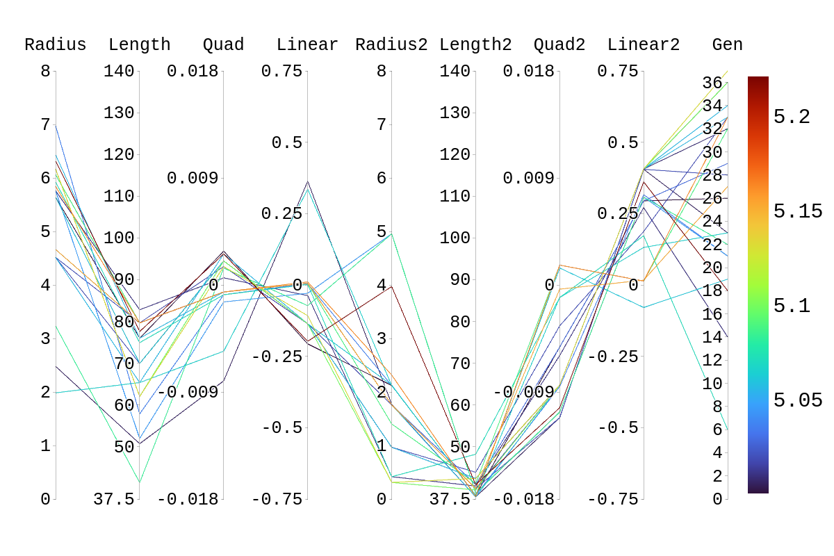
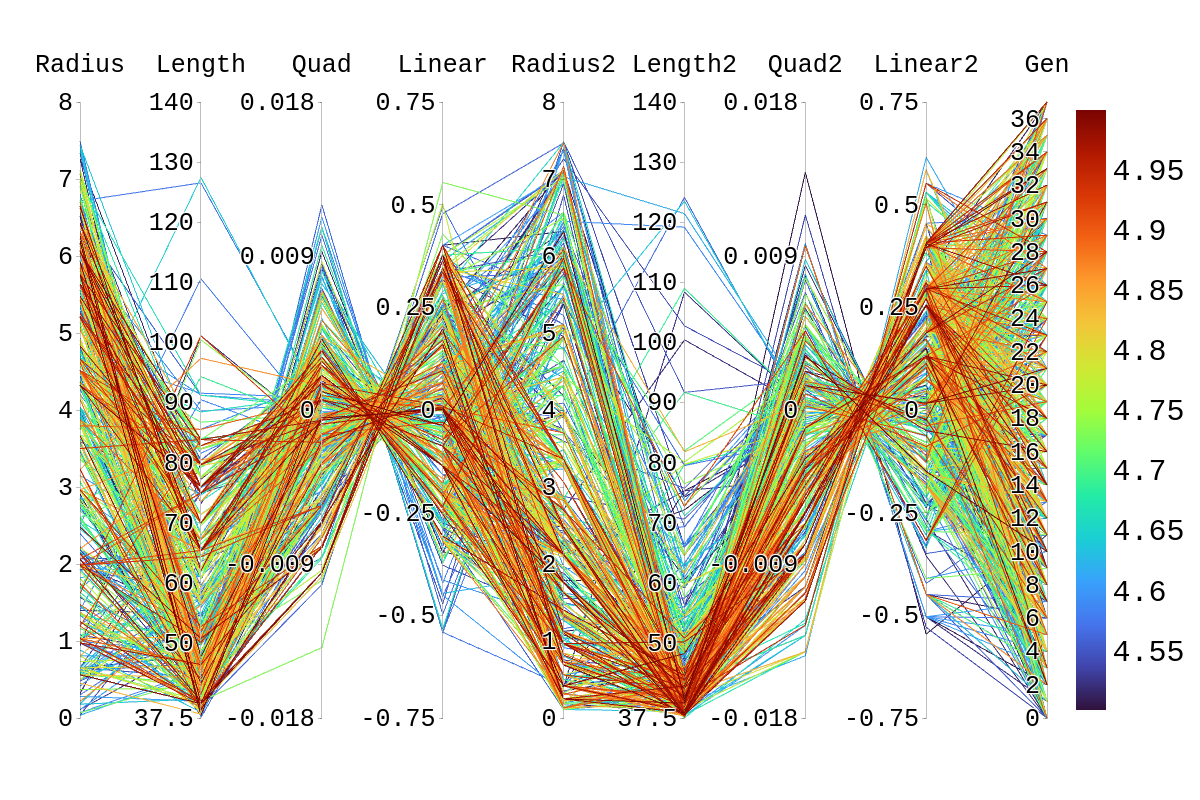
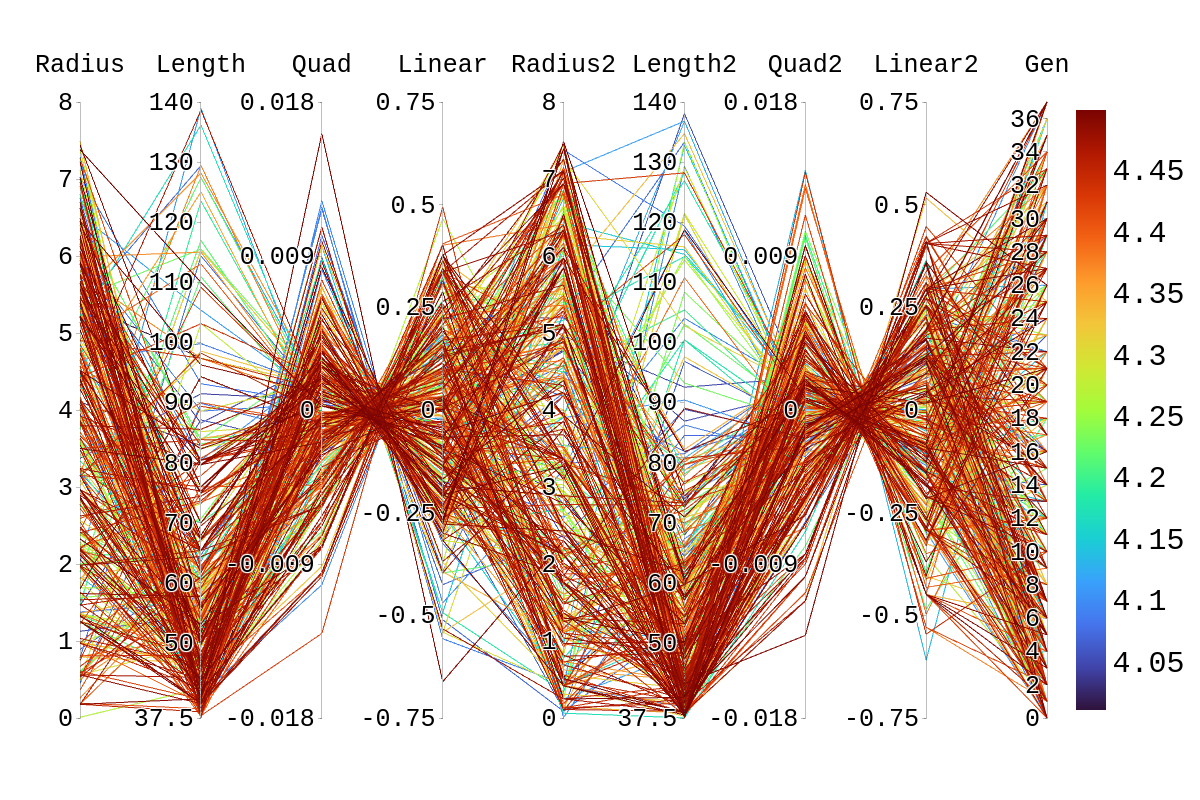
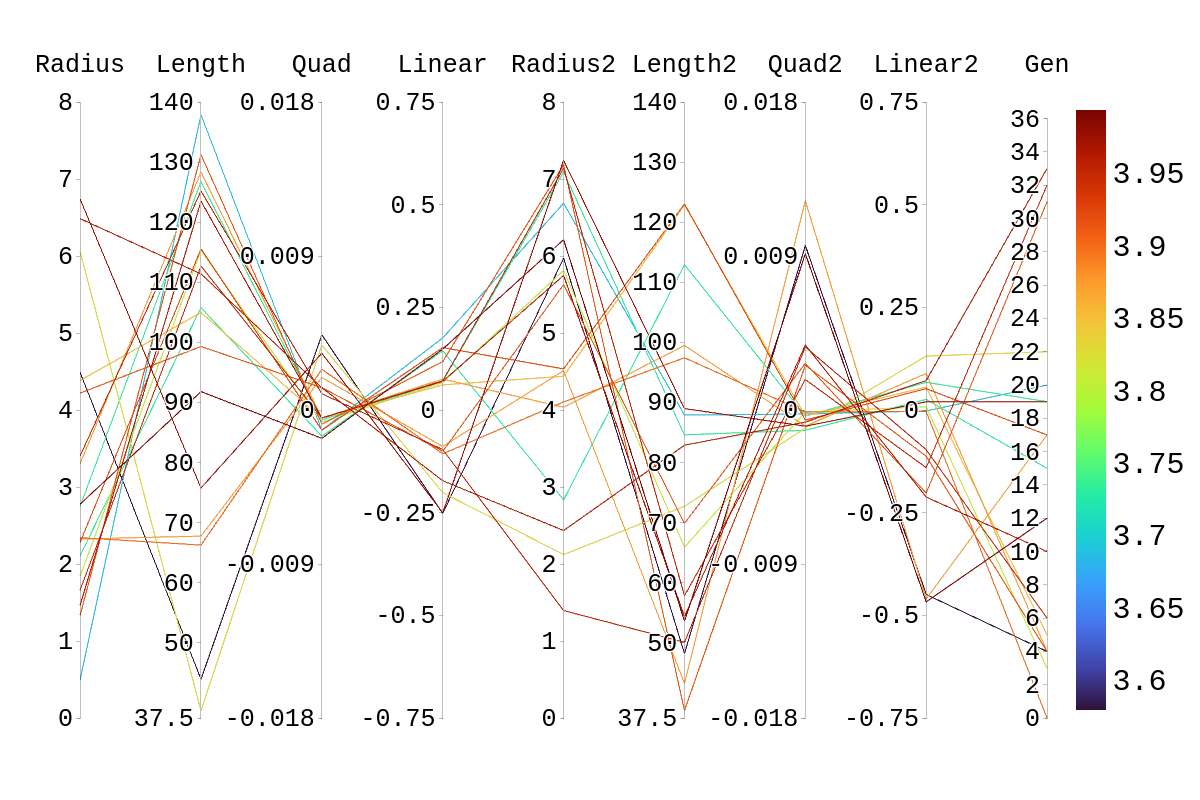
Bellow, I have attached the rainbow plot with the parameters occupied by individual 4 in gen 41 which was again ranked 39th in that generation. From this, we can see that while in its own generation it was a poor performer, overall it was upper middle of the pack. However, because of the density of other better performing antennas in this region, it is hard to distinguish which genes in this antenna are contributing the most to the drop in fitness score compared to its siblings and parents.
*Gene originating from Bicone 38.11
**Gene originating from Bicone 38.17
***Gene originating from Bicone 38.11 and 38.17 that is shared between the two. |
| Attachment 1: rainbow_plot_quadratic_rank_test_720_(drawn).png
| .png) |
|
Draft
|
Fri Jul 8 13:34:08 2022 |
Ryan Debolt | Multigenerational Narrative draft 2 | |
|
173
|
Fri Jul 8 13:35:19 2022 |
Ryan Debolt | Multigenerational Narrative draft 2 | The second-best individual in this evolution was Bicone 22 from generation 40. This individual is, in fact, a fascinating case as we shall see. But to start the story of this individual we will go back to generation 38 in order to demonstrate some of the peculiarities.
In generation 38 there were two bicones of no renown, Bicone 11 and Bicone 17. Bicone 11 was a fairly average individual that was ranked 23rd with a fitness score of 4.72016. Its DNA was {*6.16084, ***79.663, 0.0015434, -0.107765} for side one , and {0.308809, 39.6742, -0.0084247, 0.40629} for side two. One day, by chance it met Bicone 17, another average bicone ranked 24th with a score of 4.71877 and DNA {**2.32499, 79.663, -0.00224948, 0.192602} for side one, and {0.308809, 39.6742, -0.0084247, 0.40629} for side two. These two individuals eventually became the parents of two antennas: Bicone 16 and Bicone 17 of generation 39.
Bicone 16 eventually grew to have been ranked 3rd in fitness score of 4.95323. It’s DNA ended up being a complete balance of its parents sharing side one with Bicone 38.11{2.32499, 79.663, -0.00224948, 0.192602} and side two with bicone 38.17 {0.308809, 39.6742, -0.0084247, 0.40629}. Bicone 16 was an individual with high aspirations and hoped to be reproduced. But alas, it was not meant to be. But bicone 16 came upon some amazing luck, it was selected with itself for crossover. This meant that bicone 16 was able to provide two identical surrogates to survive into the next generation. This is where this Bicone fulfilled its full potential.
The twin bicones were named Bicone 22 and Bicone 23 in generation 40. Being clones, they shared all their DNA with Bicone 39.16. However, due to some circumstances, they had slightly different fitness scores. Bicone 23 managed a very respectable 5.0117 fitness score and was ranked 2nd in the generation. But not to be outdone Bicone 22 managed to score a 5.17014 and ended up being the second-best performing individual of all time. Being so successful, the two bicones ended up producing 8 children between the two groups.
Bicone 23 was the first to crossover and had 2 children with its partner Bicone 25 (4.64409). These were Bicones 4 and 5. Bicone 4 was ranked 39th with a fitness score of 4.60251 and still shared the DNA of its second side with its grandparent Bicone 38.17 as well as most of its first side with Bicone 38.11 {2.32499, 79.663, -0.00213879, 0.192602} {0.308809, 39.9608, -0.0084247, 0.40629}. Bicone 5 on the other hand, was ranked 14th with a fitness score of 4.80535 and it still shared a lot of DNA with its grandparents {6.16084,53.0851,-0.00224948,0.0534469} {0.966617,39.6742,-0.0084247,0.40629}.
Bicone 22 had 6 children of its own with various other Bicones. These were; With Bicone 8.40 (4.82423) Bicone 8, ranked 11th with a fitness Score of 4.81784 and DNA {2.32499, 75.9855, -0.00224948, 0.192602} {0.966617, 39.6742, -0.00320023, 0.213833}; Bicone 9, ranked 7th with a fitness score of 4.88966 and DNA {6.10508, 79.663, -0.000594616, 0.0351901} {0.308809, 42.4246, -0.0084247, 0.40629}; With Biocone 16.40 (5.01137) Bicone 12, ranked 12th with a fitness score of 4.81705 and DNA {6.42695, 75.9855, 0.0015434, -0.107765} {0.308809, 39.6742, -0.00320023, 0.213833}; Bicone 13, ranked 2nd with a fitness score of 5.0344 and DNA {2.32499, 79.663, -0.00224948, 0.192602} {0.966617, 42.4246, -0.0084247, 0.40629}; With Bicone 4.40 (4.66578) Bicone 34 ranked 3rd with a fitness score of 4.99864 and DNA {0.66148, 73.5522, -0.000594616, 0.00582814} {0.966617, 39.6742, -0.0084247, 0.40629}; and finally Bicone 35, ranked 22nd with fitness score 4.74955 and DNA {2.32499, 79.663, -0.00224948, 0.192602} {0.308809, 42.4246, -0.0084247, 0.40629}
Upon inspection of the children in generation 41, you will see that none of the children surpassed their parent individual with the highest fitness score. They do however tend to have fitness scores around or above their second parent's score. Therefore, it is likely that the children's lower fitness score is due to a mismatch of genes. If we look at the rainbow plots provided, we can see that the genes of the worst-performing child are not dissimilar to those of individuals that scored higher than 5. This would imply that the fitness score found could be due to variations in Arasim similar to those seen from individuals 16.39 to 22/23.40 despite them being identical. Though it also could be possible that the graphs do not have a fine enough display to be able to clearly tell some of the genes apart.
*Gene originating from Bicone 38.11
**Gene originating from Bicone 38.17
***Gene originating from Bicone 38.11 and 38.17 that is shared between the two.
Amy: We want to nail things down in places where we still have hypotheses for what could have happened. For example, "This would imply that the fitness score found could be due to variations in Arasim similar to those seen from individuals 16.39 to 22/23.40 despite them being identical. Though it also could be possible that the graphs do not have a fine enough display to be able to clearly tell some of the genes apart." These two hypotheses can easily be distinguished by running with higher statistics and looking at the numbers rather than relying on the resolution of the display.
Amy: Also, at each stage, I was looking for the random numbers that were generated that led to the selection of the fractions of the population that were used for each type of selection and operator.
|
| Attachment 1: Rainbow_Plot_Quadratic_Rank_Test_5.png
|  |
| Attachment 2: Rainbow_Plot_Quadratic_Rank_Test_4.5.png
|  |
| Attachment 3: Rainbow_Plot_Quadratic_Rank_Test_4.png
|  |
| Attachment 4: Rainbow_Plot_Quadratic_Rank_Test_3.5.png
|  |
|
176
|
Tue Aug 9 11:36:24 2022 |
Ryan Debolt | GA User guide (pdf) | |
| Attachment 1: VPol_GA_User_guide.pdf
|
|
177
|
Tue Aug 9 15:28:50 2022 |
Ryan Debolt | How many individuals to use in the GA. | One of our foundational questions tied to the optimization of the GA has been "How many individuals should we simulate". Up to now, our minds were made up for us by the speed of arasim being great enough that the time cost of simulating individuals was great enough that the improvements made from having more were not enough to justify the slowdown. However, with the upgrade to the faster, more recent version of arasim, I decided to re-examine this. This was also spurred on by the fact that the last time I ran this test we were testing GA performance by final generation metrics rather than by how many generations it took to reach a benchmark. So in one of my optimization tests, I tracked this data.
To start, using the same run proportions, using a .5 chi-squared benchmark, the average time across all 89 run types used in this run was 25.4 generations for 50 individuals as compared to 8.3 generations running the same test for 100. Furthermore, the minimum number of generations for 50 individuals was 4.8 while using 100 individuals yielded 2.4. So on average running 100 individuals was about 3 times fast at reaching this benchmark than with 50. And when comparing the best result regardless of run type, 100 individuals was still 2 times quicker than the min for 50 individuals. Finally, the run that yielded an average of 2.4 generations for 100 individuals took an average of 29.2 generations with 50 individuals or roughly 12 times the generations.
For the test we will discuss, we ran 89 different run types that all used 60% rank, 20% roulette, and 20% tournament selection respectively. These test had the following ranges:
6-18% of individuals through reproduction (steps of 3%)
64-88% of individuals through crossover (steps of 12%)
0-10% mutation rate (steps of 5%)
1-5% sigma on mutation (steps of 1%)
These tests also used our fitness scores with simulated error of .1 to imitate arasim's behavior and as such we used the chi-squared value to evaluate these scores as there is no error on those values.
Comparing this same test with a tighter chi-squared benchmark of .25, we see similar results. On average 50 individuals took 37.1 generations to reach this point while 100 individuals took 16.0 generations. Similarly, the minimums amount of gens for 50 individuals was 15.4 while 100 individuals was 5. Finally, the corresponding run for the 5 generation min with 100 individuals took 41.8 generations with 50 individuals. These correspond to speed up's of 2.3, 3.08, and 8.36 respectively.
This data implies that on average, independent of run type, we should expect to have to use 2-3 times fewer generations while running 100 individuals than we would running 50 individuals but we could see up to 8-12 times fewer generations to reach benchmarks. Another data set using a different set of selection methods was also tested for this and again yielded similar results, though overall the runs from the first batch were better across both 50 and 100 individuals and so those results are likely to be more indicative of the parameters we use in a true run.
The data being examined in these results can be found here: https://docs.google.com/spreadsheets/d/1GlfnjQSO6VI8MuUGYTUcLkjwDZU98nyFFysgTTfVFOE/edit?usp=sharing |
|
Draft
|
Mon Oct 24 17:44:51 2022 |
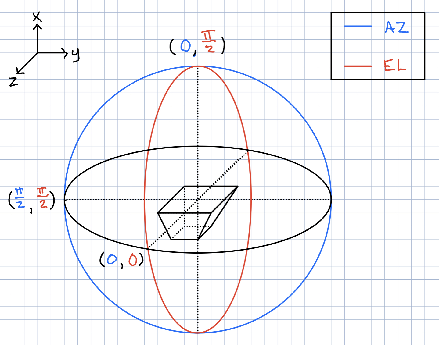
Ryan Debolt | Icemc inputs | Here is our current assumption of the antenna angles needed for the icemc inputs. |
| Attachment 1: 261D6FA3-5612-412F-80FA-8AD961F7331A.jpeg
|  |
|
185
|
Thu Nov 10 10:42:20 2022 |
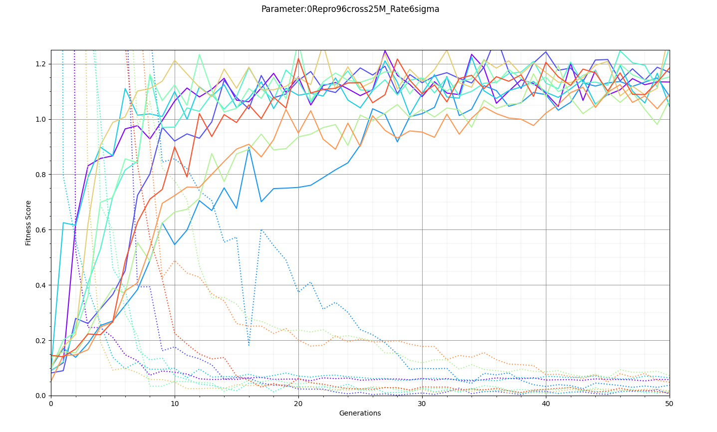
Ryan Debolt | Optimizations | This is the plot for the run type that had the best performance in the most recent optimization run that was completed. The most optimized runs from these collections are decided by which run types achieve a chi-squared value of 0.1 in the fewest generations (correlating to about a 0.9 fitness score). However, the genetic algorithm does not use Chi-squared directly, instead trying to maximize the fitness score (which uses a chi-squared in the denominator) that simulates the error we see in arasim. This fitness score is usually maximized at 1.0 but the simulated error can push the score slightly beyond this. This test was conducted with a simulated error of 0.1. This optimization holds the selection methods steady at 2 tournament 2 roulette and 6 rank selected individuals per 10 selection events. The changing parameter values are in the amounts of Reproduction, Crossover, Immigration, and mutation (rate and width) that the GA performs each generation. Each generation uses 100 individuals. In the graph below, the dotted lines are the minimum Chi^2 values at each generation, solid lines are the maximum fitness score. Each color represents a different run using the same parameters and dotted and solid lines sharing the same color represent the same run. The prevailing trend in the tests leading up to this test has been that the most optimized runs have low amounts of reproduction, high amounts of crossover, and they have been pushing the boundaries of the mutation rate and gaussian width of those mutations and this run follows that trend. The ranges of values we tested over were 0-12R, 88-100C, 15-25M_Rate, and 3-7 sigma, up from the previous test. This run took an average of 16.8 +/- 11.9 generations to reach the 0.1 chi-squared benchmark, the next closest run took 20.3 +/- 10.9 generations to reach the same point, while the most optimized run from an earlier test came in as the 10th best run taking 21.9 +/- 14.4 generations. The graph shows the behavior of this by showing large improvements in early generations that tend to quickly plateau around the maximum value before oscillating around the peak it reaches. Oscillations could be caused by either small mutations around our answer and displacement from the simulated error. The Chi-squared values show a much smoother behavior with smaller oscillations at the end of the run, which helps demonstrate the impact of the error on the behavior. |
| Attachment 1: Plot0_96_25_6.png
|  |
|
223
|
Fri Jun 2 00:21:36 2023 |
Ryan Debolt | Error test results | Attached is a plot containing bar graphs with error bars representing the average number of generations it took for the GA to achieve a chi-squared value of 0.25 (roughly equated to a 0.8 out of a max 1.0 fitness score). Unlike the fitness scores used by the GA, these values do not have simulated error attached to them and are therefore a better measure of how well the GA is optimizing. These results were obtained by running 10 tests in the test loop for each design, population, and error combination and solving for the average number of generations to meet our threshold and the standard deviation of those scores. From this, a few things immediately pop out, I will address the more obvious one later. But essential for this test, we can see that increasing our population size seems to have a more direct impact on the number of generations needed to reach our threshold than decreased error does in both designs. My best guess regarding this is that the GA depends on diversity in its population in order to produce efficient growth, and an increase in the number of individuals contributes to this, allowing the GA to explore more options.
This leads me to the more easily spotted trend; PUEO is much slower than ARA. This presents an anomaly as this is the opposite of what we would expect from this test loop as PUEO has fewer genes (7) to optimize than ARA (8). It is also important to note that no genes are being held constant in this test for either design, so both designs have the full range of designs provided they are within the constraints. With that in mind, my guess as to what causes this phenomenon is that PUEO's constraints are much stronger than ARA's. How this may affect the growth is that it more heavily bounds the possible solutions, which makes it harder for the GA to iterate on designs. It is possible that during a function like a crossover, the only possible combinations for a pair of children are identical to their parents, effectively performing reproduction. This could limit the genetic diversity in a population and therefore cause an increase of generations needed to reach an answer. We could in theory test this by relaxing the constraints done by PUEO and then running the test again to see how it compares.
Finally, You will notice that no AREA designs are shown. This is because, under current conditions, they never reached the threshold within 50 generations. However, Bryan and I think we know what is happening there. AREA has 28 genes, about four times the amount of genes that our other designs use. Given that our current test loop fitness measure is dependent on a chi-squared value given by: SUM | ((observed(gene) - expected(gene))^2) / expected(gene) |, we can see that given more genes, the harder it gets to approach zero. For example, we can imagine in an ARA design if each index of the sum equals 0.1, you would get a total value of 0.8, while AREA would get a value of 2.8, which seems considerably worse, despite each index being the same. Upon further thinking about it, Bryan and I do not think that a chi-squared is the best measure of fit we could be using in this context. Another thing we thought about is that we have negative expected values in some cases. We have skirted around this by using absolute values, but upon reflection believe this to be an indicator of a poor choice in metric. Chi-Squared calculations seem to be a better fit for positive, independent, and normally distributed values, rather than our discrete values provided by our GA. With this in mind, we propose changing to a Normalized Euclidean Distance metric to calculate our fitness scores moving forward. This is given by the calculation: d = sqrt((1/max_genes) * SUM (observed(gene) - expected(gene))^2). This accomplishes a few things. First, it keeps the same 0 -> infinity bounds that our current measure has, allowing our 1/(1+d) fitness score to be bounded between 0 and 1. Second, it forces all indices to be positive so we don't need to worry about negative values in the calculation. Third, this function is weighted by the number of genes present for any given design, making them easier to compare than our current measure. Finally, as our GA is technically performing a search in an N-dimensional space for a location that provides a maximized fitness score, it makes sense to provide it the distance a solution is from that location as a measure of fit in our test loop. We created a branch on the test loop repository to test this and the results are promising as results from the three designs are much more comparable for the most part (though we still see some slowdown we think is contributed to constraints as mentioned above). Though some further input would be appreciated before we begin doing tests like the one we have done in the plot below. |
| Attachment 1: test_results(1).png
| .png) |
|