| ID |
Date |
Author |
Type |
Category |
Subject |
Project |
|
12
|
Thu Mar 23 20:08:52 2017 |
J. C. Hanson | Analysis | Analysis | Latest near-surface ice report | | Hello! See the attached report relating the compressibility of firn, the density profile, and the resulting index of refraction profile. The gradient of the index of refraction profile determines the curvature of classically refracted rays. |
| Attachment 1: NearSurface_IceReport.pdf
|
|
13
|
Thu Mar 23 21:43:12 2017 |
Abdullah Alhag | Analysis | Analysis | The results from running Karoo on the inelasticity data | | See attatchd file. |
| Attachment 1: The_result_of_using_Karoo_on_inelasticity_data.pdf
|
|
18
|
Wed Jul 5 19:22:52 2017 |
Brian Clark and Ian Best | Lab Measurement | Hardware | Mac Addresses | | This is a "bank" of mac addresses that we obtained for the lab. They were taken by Ian Best (one of Jim' students) in summer 2017. We purchased 25 AT24MAC402 EEPROMS (https://www.arrow.com/en/products/at24mac402-stum-t/microchip-technology) and used a SOT-23 breakout board and a bus pirate to retrieve their internal mac addresses.
If you take one, please note where you used it so no one tries to take the same one twice:
| Serial Number |
EUI (Mac) Address |
Used? |
| 0x0A70080064100461105CA000A0000000 |
FC:C2:3D:0D:A6:71 |
Spare ADAQ (ADAQF002) |
| 0x0A70080064100460FC6DA000A0000000 |
FC:C2:3D:0D:A7:37 |
Spare ADAQ (ADAQF003) |
| 0x0A700800641004611C8DA000A0000000 |
FC:C2:3D:0D:A8:7C |
Spare ADAQ (ADAQF004) |
| 0x0A70080064100461E47FA000A0000000 |
FC:C2:3D:0D:BC:BF |
-- reserved for testing |
| 0x0A700800641004611C9FA000A0000000 |
FC:C2:3D:0D:BE:02 |
|
| 0x0A70080064100461D8D9A000A0000000 |
FC:C2:3D:0D:C0:2D |
|
| 0x0A700800641004611C6EA000A0000000 |
FC:C2:3D:0D:C6:62 |
|
| 0x0A70080064100460F0A0A000A0000000 |
FC:C2:3D:0D:C8:AF |
|
| 0x0A70080064100461F870A000A0000000 |
FC:C2:3D:0D:DC:22 |
|
| 0x0A700800641004612CC7A000A0000000 |
FC:C2:3D:0D:E9:F4 |
ARA3 ADAQ (ADAQG003) |
| 0x0A70080064100461EC43A000A0000000 |
FC:C2:3D:0D:EF:78 |
|
| 0x0A7008006410046228B7A000A0000000 |
FC:C2:3D:0D:FE:3D |
|
| 0x0A70080064100461F065A000A0000000 |
FC:C2:3D:0E:05:6F |
|
| 0x0A70080064100461E8CDA000A0000000 |
FC:C2:3D:0E:14:4F |
|
| 0x0A70080064100461E07AA000A0000000 |
FC:C2:3D:0E:3A:AB |
ARA6 ADAQ (ADAQG004) |
| 0x0A700800641004611813A000A0000000 |
FC:C2:3D:0E:6B:08 |
|
| 0x0A700800641004612014A000A0000000 |
FC:C2:3D:0E:6B:59 |
|
| 0x0A70080064100461E415A000A0000000 |
FC:C2:3D:0E:75:AE |
|
| 0x0A70080064100461F034A000A0000000 |
FC:C2:3D:0E:CB:03 |
PUEO TURF 2 (rsvd) |
| 0x0A700800641004623434A000A0000000 |
FC:C2:3D:0E:CB:23 |
PUEO TURF 2 (main) |
| 0x0A70080064100462A037A000A0000000 |
FC:C2:3D:0E:D5:55 |
PUEO TURF 1 (rsvd) |
| 0x0A700800641004610C0DA000A0000000 |
FC:C2:3D:0E:E9:4A |
PUEO TURF 1 (main) |
| 0x0A70080064100461E825A000A0000000 |
FC:C2:3D:0E:E9:DC |
PUEO TURF 0 (rsvd) |
| 0x0A700800641004617438A000A0000000 |
FC:C2:3D:0E:EA:9E |
PUEO TURF 0 (main) |
|
|
20
|
Fri Jul 28 17:43:20 2017 |
Abdullah Alhag | Analysis | Analysis | GP algorithms | | In this post, I will be pointing out the advantage and the disadvantage of the GP algorithms I came across, particular Eureqa and HeuristicLab.
Eureqa is by far the fastest genetic algorithm software I came across. It is over simplified and easy to use. It has some built-in fitness function and also with some playing with the function that is being solved for and some other feature, it is possible for one to write his/her own fitness function. Moreover, the software is available for free for academic use and for most platform. Other features come with the software is the ability to normalize the data in different ways and even handle outliers and missing data. The program support a large collection of functions including trig and more complex one.
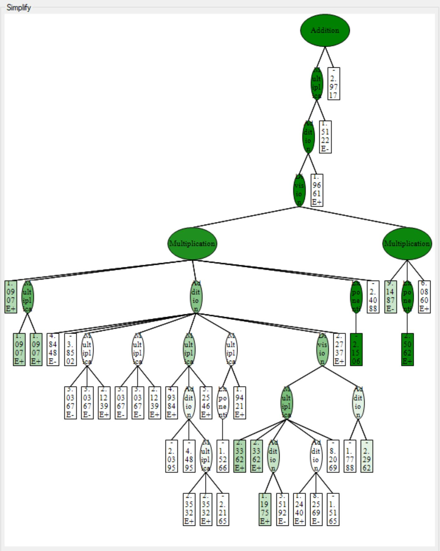
One the other hand, HeuristicLab is much slower than Eureqa but still far faster than Karoo-GP. The latest version of the software was released a year ago, and the support for the software is fairly slow. It is only supported for Windows; however, there is plans to adopted to Linux systems. The software support way more feature than Eureqa or karoo and even different regression and classification algorithms. You could also get the function ready to use in many software such as MATLAB, Excel, Mathematica, and much more. Another cool feature is that it shows you a three of the function and the weight of each node (operation or operand), greener means the node has more weight, see attached. It should be noticed that the software has the tendency to grow large three which could be fixed by changing the default max three length and the max three depth. The software has a problem with the last update of windows 10, you will get the blue screen if you opened too many windows, so be careful.
In booth software you could change how much of the data set goes to training and how much goes to testing, be sure to shuffle the data in HeuristicLab as it will otherwise distribute the data as training and testing non-randomly. Booth software by default shows plot of the current function with the x axis being the data entries (row numbers) and y axis being the target values with a curve of the function estimate values.
Below is a simple run of both software on a fake data that Prof. Amy gave me, see out.txt for data.
For start, using eureqa I got a few functions with an average of mean of R^2 of 0.98 or more which is very good.
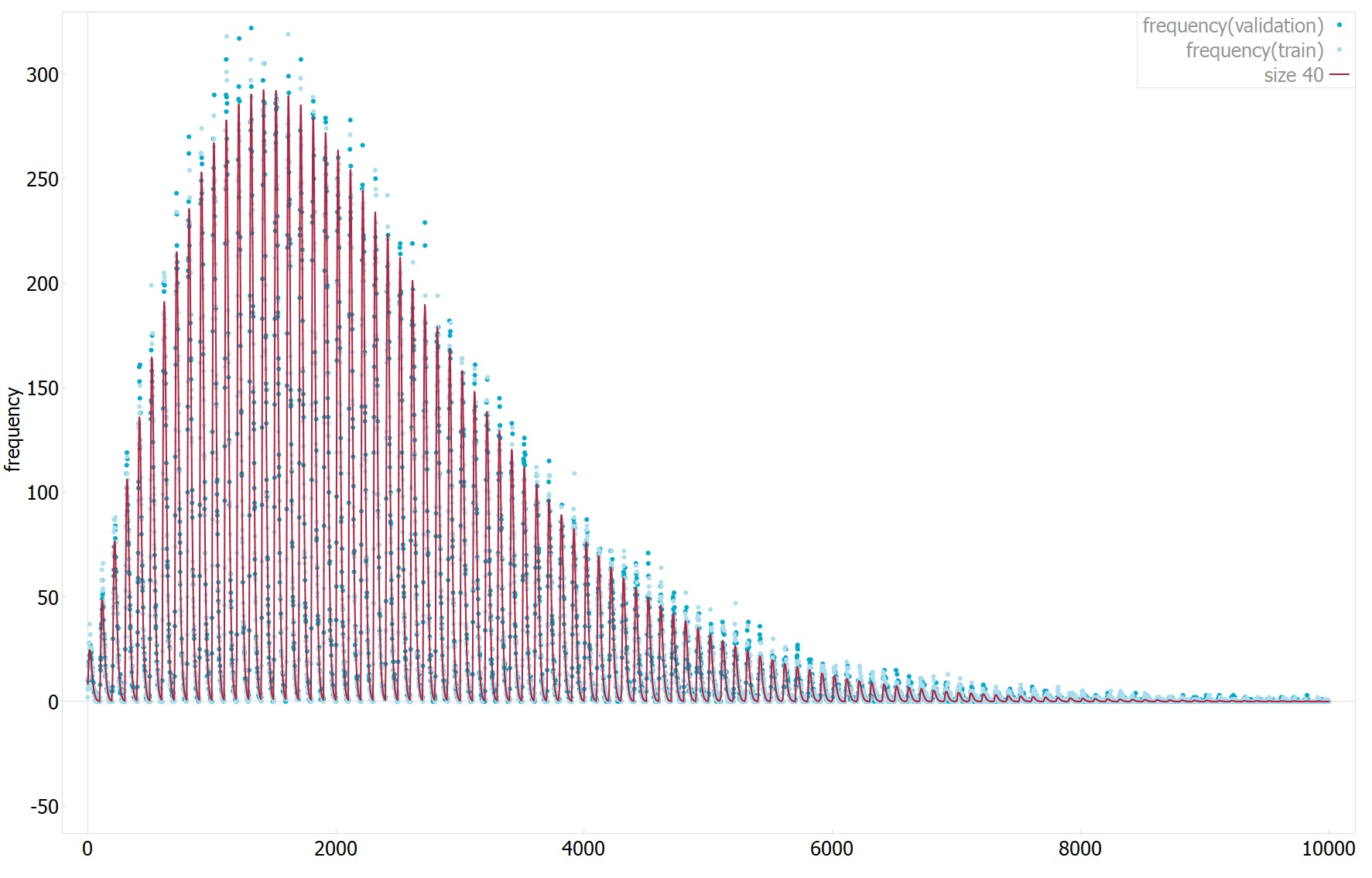
First function: frequency = (571953.335547372*y + 15786079*x^2*y^4 + 297065746*x*y^2*asinh(x))/factorial(7.44918899410674 + x + y)
The first has an R^2 of 0.99(1 means perfect fit) and mean absolute error of 2.98(0 means perfect fit, data dependent, not normalized), see plot1 for 1D plot of the function estimate values vs target values.
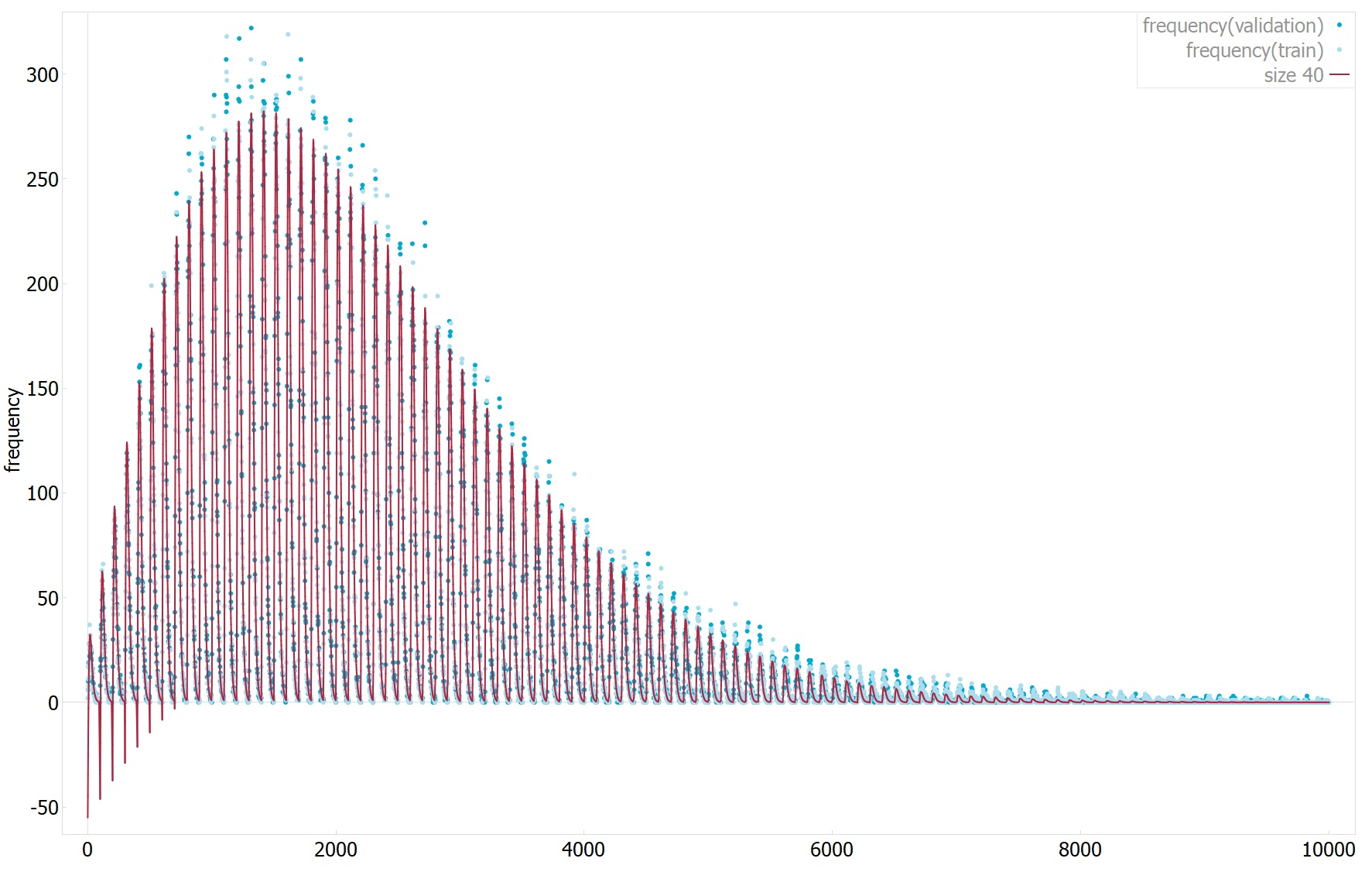
Second function: frequency = (3569.91823898791*x*y - 149.144996501988 - 100.216589664235*x^2)/(5.26462242203202^x + 7.09216771444399^y*x^(1.3193170267439*x))
The second has an R^2 of 0.994(1 means perfect fit) and mean absolute error of 3.2(0 means perfect fit, data dependent, not normalized), see plot2 for 1D plot of the function estimate values vs target values.
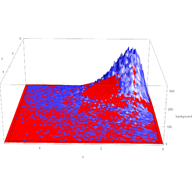
Also attached is 2D plot of the function against the data, the function plotted is the second function, but all are very similar, see Eq23.
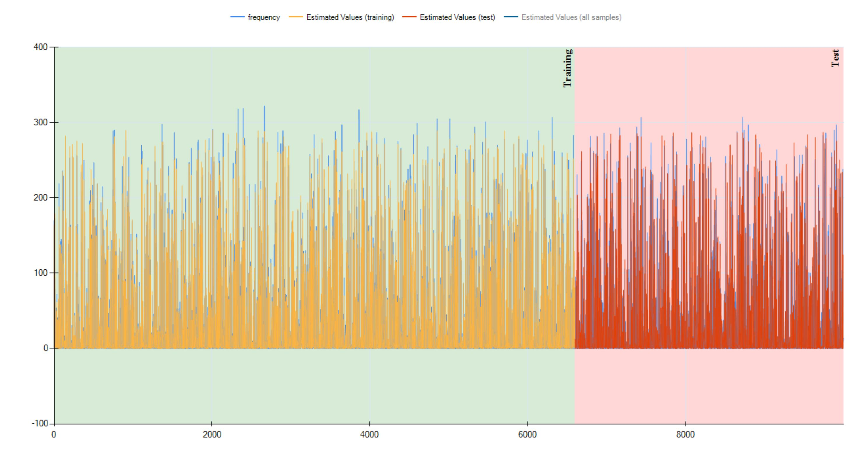
Using HeuristicLab. The function below has an R^2 of 0.987, mean absolute error of 3.6 and normalized mean squared error of 0.012.
The function is: (((EXP((-1.3681014170483*'y')) * ((((-1.06504220396658) * (2.16142798579652*'x')) * (3.44831687407881*'y')) / ((((1.57186418519305*'y') + (2.15361749794796*'y')) / ((1.6912208581006*'y') / (EXP((1.80824695345446*'x')) * 16.3366330774664))) / ((((2.11818004168659*'x') * (1.10362178478116*'y')) - ((((-1.06504220396658) * (2.16142798579652*'x')) * (3.44831687407881*'y')) / ((((2.11818004168659*'x') + (2.15361749794796*'y')) / ((10.9740866421104 + (1.8106235953875*'y')) - (2.15361749794796*'y'))) / (((-7.8798958167) + (-6.76475761634751)) + ((2.87007061579651*'x') + (2.15361749794796*'y')))))) - (((((-8.85637334631747) * ((1.9238243855142*'y') - (1.01219957177297*'y'))) + (((-6.37085286789103) * 5.99856391145622) - ((-12.9565240969832) - 2.84841224458228))) - ((2.11818004168659*'x') * (1.10362178478116*'y'))) - (((2.11818004168659*'x') * ((((0.197306324191089*'y') + (0.255996267596584*'y')) - (2.16142798579652*'x')) - (((-1.06504220396658) * (2.16142798579652*'x')) / (12.2597910897177 / (1.25729305246107*'y'))))) - (EXP((-1.3681014170483*'y')) - ((((-6.29806655709512) * 6.39744830364858) / (12.2597910897177 / (0.728256926023423*'x'))) - (1.10362178478116*'y'))))))))) * 179.42788632856) + 2.24688690162535)
As you could see, HeuristicLab tend to generate function which are extremely large, this one has a depth of 15 and a length of 150.
See plot3 for 1D plot of the function estimate values vs target values, note that it is different from before because the data is shuffled, and three.jpg for the three representation of the function showing the wight of each node, greener means has more weight. |
| Attachment 1: plot1.png
|  |
| Attachment 2: plot2.png
|  |
| Attachment 3: plot3.png
|  |
| Attachment 4: Eq23-0.png
|  |
| Attachment 5: three.png
|  |
|
24
|
Sun Sep 17 20:10:21 2017 |
Spoorthi Nagasamudram | Modeling | Simulation | A different way to implement ray tracing in AraSim (possibly even other simulations) | | Hi,
I've attached a copy of some of the work I did over the summer on ray tracing and how I did it. Please let me know if you have any questions.
PS The plots are sidewards for some reasons. Sorry about that.
|
| Attachment 1: raytracing_elog.pdf
|
|
29
|
Tue Feb 27 23:13:15 2018 |
Amy Connolly | Other | Simulation | Plots for QC sites | | Hi All,
We need to revive the icemcQC and AraSimQC pages, and I thought that in the meantime we could keep a list and/or associated code for plots we'd like to see go in there.
Here are a couple plots I just made code attached is forstevenanddave.cc
event weight (attenuation factor) vs. angle that neutrino makes wrt up when standing under the anita balloon
event weight (attenuation factor) vs. angle that rf makes wrt up from an observer on the anita balloon
BC: Adding old Stephen Hoover plots from ANITA elog: https://www.phys.hawaii.edu/elog/anita_notes/32
|
| Attachment 1: forstevenanddave.cc
|
#include <iostream>
#include <fstream>
#include <math.h>
#include <string>
#include <stdio.h>
#include <stdlib.h>
#include <vector>
#include <time.h>
//#include <cmath>
#include "TH1.h"
#include "TFile.h"
#include "TLine.h"
#include "TTree.h"
#include "TROOT.h"
#include "TPostScript.h"
#include "TCanvas.h"
#include "TH2F.h"
#include "TText.h"
#include "TProfile.h"
#include "TGraphErrors.h"
#include "TRandom.h"
#include "TRandom2.h"
#include "TRandom3.h"
#include "TStyle.h"
#include "TVector3.h"

using namespace std;

TStyle* RootStyle();
TStyle *color=RootStyle();

double PI=3.1415926;

double R_EARTH=6.36E6;

TRandom3 *Rand3=new TRandom3();


int main(int argc, char *argv[]) {

  gStyle=color;
  gStyle->SetPalette(1);

  TFile *f = new TFile("/Users/amyc/icemc/outputs/icefinal.root");
  TTree *t1 = (TTree*)f->Get("passing_events");
  double logweight,theta_in,costhetanu,cosalpha,phi_in;
  double theta_rf_atbn;
  double e_component,h_component;
  double weight;

  t1->SetBranchAddress("logweight",&logweight);
  t1->SetBranchAddress("weight",&weight);
  // t1->SetBranchAddress("theta_in",&theta_in);
  //t1->SetBranchAddress("phi_in",&phi_in);
  //t1->SetBranchAddress("costhetanu",&costhetanu);
  t1->SetBranchAddress("cosalpha",&cosalpha);
  t1->SetBranchAddress("theta_rf_atbn",&theta_rf_atbn);
  t1->SetBranchAddress("e_component",&e_component);
  t1->SetBranchAddress("h_component",&h_component);

  TH2D *h2_weight_thetarf=new TH2D("h2_thetarf","h2_thetarf",100,50.,100.,100,-10.,1.);
  TH2D *h2_weight_alpha=new TH2D("h2_alpha","h2_alpha",100,90.0,130.,100,-10.,1.);
  TH1D *h2_ratio=new TH1D("h2_ratio","h2_ratio",100,-20.0,20.);

  for (int i=0;i<t1->GetEntries();i++) {
    t1->GetEvent(i);

    h2_weight_thetarf->Fill(theta_rf_atbn*180./PI,logweight);
    h2_weight_alpha->Fill(acos(cosalpha)*180./PI,logweight);
    h2_ratio->Fill(e_component/h_component,1E5*weight);
    cout << "weight, theta are " << logweight << "\t" << theta_rf_atbn << "\n";
  }

  TCanvas *c1=new TCanvas("c1","c1",800,800);
  c1->Divide(1,2);

  h2_weight_thetarf->SetXTitle("#theta_{rf at bn}");
  h2_weight_thetarf->SetYTitle("Weight");

  c1->cd(1);
  h2_weight_thetarf->SetMarkerSize(0.5);
  h2_weight_thetarf->Draw();

  c1->cd(2);
  h2_weight_alpha->SetXTitle("#theta_{#nu wrt up}");
  h2_weight_alpha->SetYTitle("Weight");
  h2_weight_alpha->Draw();

  c1->cd(2);
  h2_weight_alpha->SetXTitle("#alpha_{rf at bn}");
  h2_weight_alpha->SetYTitle("Weight");
  h2_weight_alpha->Draw();


  c1->Print("stevenanddave.eps");

  return 0;

}


TStyle* RootStyle() {

  //  const char* modified = "Borrowed and adapted from paus et al";

  TStyle *RootStyle = new TStyle("Root-Style","The Perfect Style for Plots ;-)");

#ifdef __CINT__
  TStyle *GloStyle;
  GloStyle = gStyle;                          // save the global style reference

  gStyle = RootStyle;
#endif
// otherwise you need to call TROOT::SetStyle("Root-Style")

  // Paper size

  RootStyle->SetPaperSize(TStyle::kUSLetter);

  // Canvas

  RootStyle->SetCanvasColor     (0);
  RootStyle->SetCanvasBorderSize(10);
  RootStyle->SetCanvasBorderMode(0);
  RootStyle->SetCanvasDefH      (600);
  RootStyle->SetCanvasDefW      (600);
  RootStyle->SetCanvasDefX      (10);
  RootStyle->SetCanvasDefY      (10);

  // Pads

  RootStyle->SetPadColor       (0);
  RootStyle->SetPadBorderSize  (10);
  RootStyle->SetPadBorderMode  (0);
  //  RootStyle->SetPadBottomMargin(0.13);
  RootStyle->SetPadBottomMargin(0.16);
  RootStyle->SetPadTopMargin   (0.08);
  RootStyle->SetPadLeftMargin  (0.15);
  RootStyle->SetPadRightMargin (0.15);
  RootStyle->SetPadGridX       (0);
  RootStyle->SetPadGridY       (0);
  RootStyle->SetPadTickX       (1);
  RootStyle->SetPadTickY       (1);

  // Frames

  RootStyle->SetFrameFillStyle ( 0);
  RootStyle->SetFrameFillColor ( 0);
  RootStyle->SetFrameLineColor ( 1);
  RootStyle->SetFrameLineStyle ( 0);
  RootStyle->SetFrameLineWidth ( 2);
  RootStyle->SetFrameBorderSize(10);
  RootStyle->SetFrameBorderMode( 0);


  // Histograms

  RootStyle->SetHistFillColor(0);
  RootStyle->SetHistFillStyle(1);
  RootStyle->SetHistLineColor(1);
  RootStyle->SetHistLineStyle(0);
  RootStyle->SetHistLineWidth(2);

  // Functions

  RootStyle->SetFuncColor(1);
  RootStyle->SetFuncStyle(0);
  RootStyle->SetFuncWidth(1);

  //Legends

  RootStyle->SetStatBorderSize(2);
  RootStyle->SetStatFont      (42);
  //  RootStyle->SetOptStat       (111111);
  RootStyle->SetOptStat       (0);
  RootStyle->SetStatColor     (0);
  RootStyle->SetStatX         (0.93);
  RootStyle->SetStatY         (0.90);
  RootStyle->SetStatFontSize  (0.07);
  //  RootStyle->SetStatW         (0.2);
  //  RootStyle->SetStatH         (0.15);

  // Labels, Ticks, and Titles

  RootStyle->SetTickLength ( 0.015,"X");
  RootStyle->SetTitleSize  ( 0.055,"X");
  RootStyle->SetTitleOffset( 1.00,"X");
  RootStyle->SetTitleBorderSize(0);
  //  RootStyle->SetTitleFontSize((float)3.);
  RootStyle->SetLabelOffset( 0.015,"X");
  RootStyle->SetLabelSize  ( 0.050,"X");
  RootStyle->SetLabelFont  ( 42   ,"X");

  RootStyle->SetTickLength ( 0.015,"Y");
  RootStyle->SetTitleSize  ( 0.055,"Y");
  RootStyle->SetTitleOffset( 1.300,"Y");
  RootStyle->SetLabelOffset( 0.015,"Y");
  RootStyle->SetLabelSize  ( 0.050,"Y");
  RootStyle->SetLabelFont  ( 42   ,"Y");

  RootStyle->SetTitleFont  (42,"XYZ");
  RootStyle->SetTitleColor  (1);

  // Options

  RootStyle->SetOptFit     (1);

  RootStyle->SetMarkerStyle(20);
  RootStyle->SetMarkerSize(0.8);

  //  cout << ">> Style initialized with the Root Style!" << endl;
  //  cout << ">> " << modified << endl << endl;
  return RootStyle;
}
//need to get expected limit with sprinkling (counting exp and binned), observed limit given the two observed in the bins we saw them, observed limit including clustered events in passing events.  try to do the same for dailey's?
|
| Attachment 2: plot_note.ps
|
|
Draft
|
Sat Apr 18 21:16:34 2026 |
Amy Connolly | Other | Simulation | Plots for QC sites | |
| Quote: |
|
Hi All,
We need to revive the icemcQC and AraSimQC pages, and I thought that in the meantime we could keep a list and/or associated code for plots we'd like to see go in there.
Here are a couple plots I just made code attached is forstevenanddave.cc
event weight (attenuation factor) vs. angle that neutrino makes wrt up when standing under the anita balloon
event weight (attenuation factor) vs. angle that rf makes wrt up from an observer on the anita balloon
BC: Adding old Stephen Hoover plots from ANITA elog: https://www.phys.hawaii.edu/elog/anita_notes/32
|
|
|