| |
ID |
Date |
Author |
Subject |
|
|
Draft
|
Mon Apr 24 13:09:36 2023 |
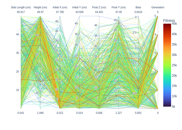
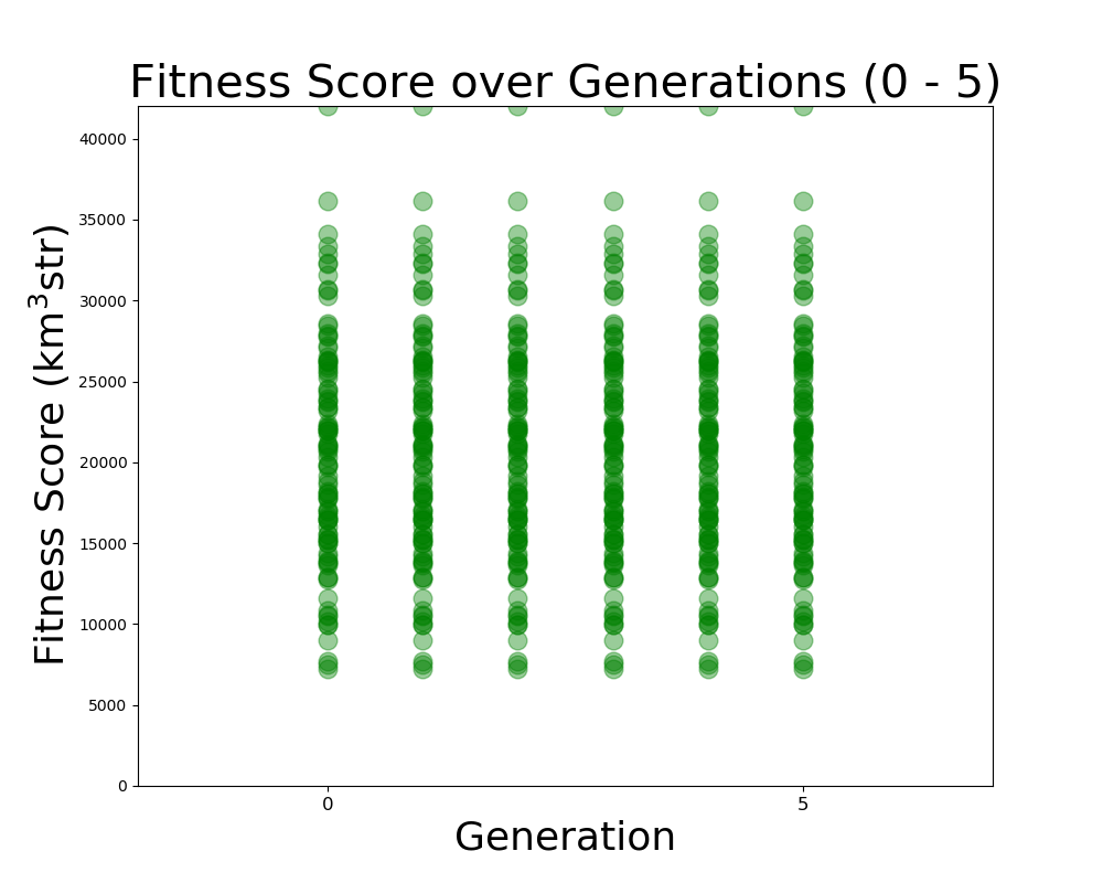
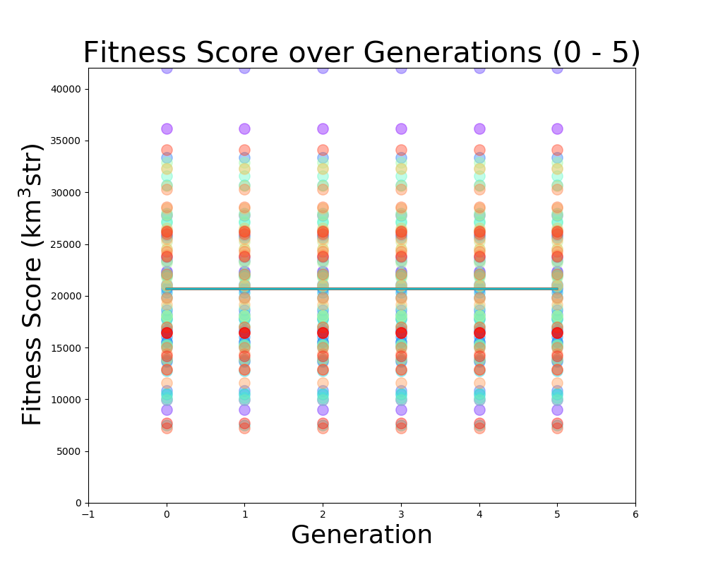
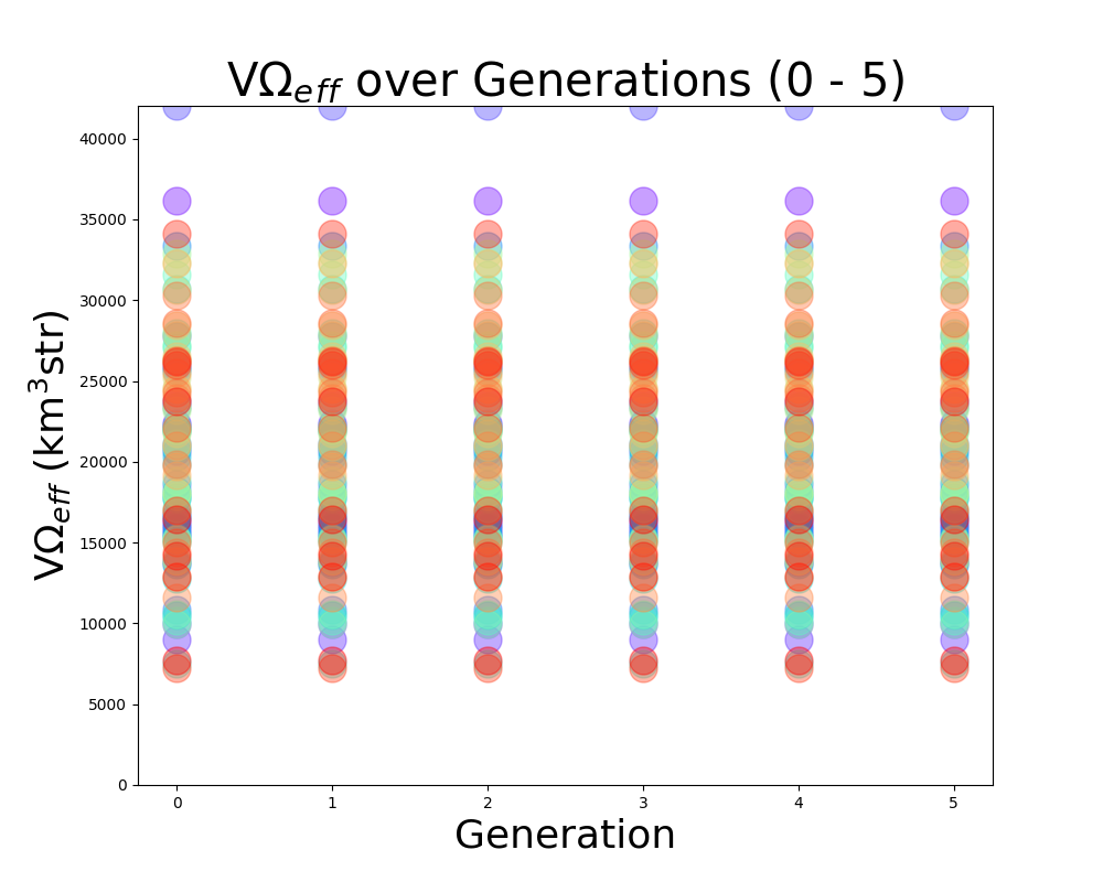
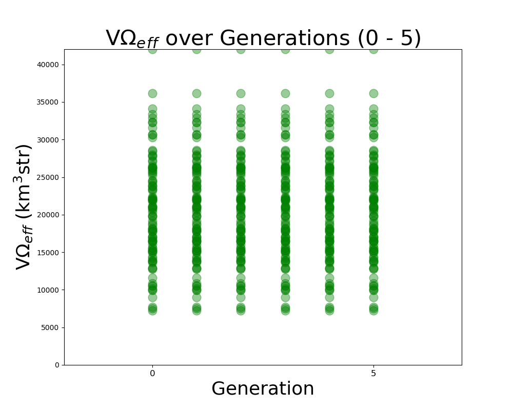
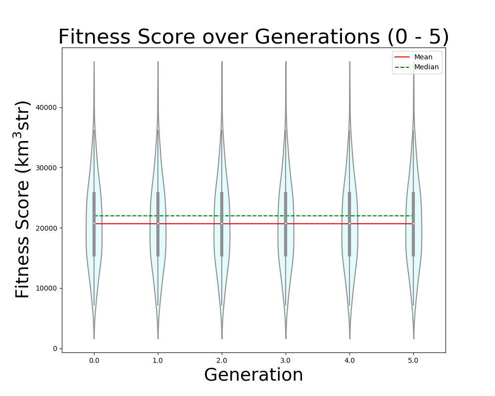
Dylan Wells | PUEO Plots Status | Plots we want to have for PUEO:
FScorePlot2D
Fitness_Scores_RG
VariablePlot (PUEO equivalent of LRT plot)
Veff_Plot (currently the veff is equivalent to the fitness score for PUEO)
Veffectives_RG
Rainbow_Plot
Violin Plot
avg_freq
gain_vs_freq
polar_plotter
physics of results
Next steps:
Get the Error values out of the pueoSim root output (talking to Will)
Use output uan files from the new two-run XF simulation to test the frequency plots. (/fs/ess/PAS1960/HornEvolutionOSC/GENETIS_PUEO/BiconeEvolution/current_antenna_evo_build/XF_Loop/Evolutionary_Loop/Run_Outputs/2023_04_21_Test_6)
Implement the physics of results plots into the loop (Talk to Bryan / Dennis)
Get the average Veff/Fitness score from the default gain pattern in pueoSim to compare our results to. |
| Attachment 1: Rainbow_Plot.png
|  |
| Attachment 2: VariablePlot.png
|  |
| Attachment 3: Fitness_Scores_RG.png
|  |
| Attachment 4: FScorePlot2D.png
|  |
| Attachment 5: Veff_plot.png
|  |
| Attachment 6: Veffectives_RG.png
|  |
| Attachment 7: ViolinPlot.png
|  |
|
|
Draft
|
Tue Apr 11 00:36:49 2023 |
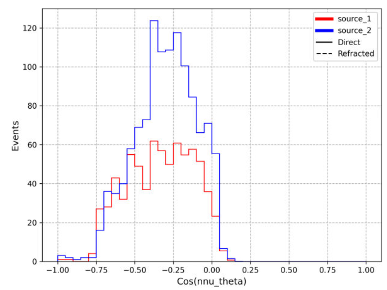
Bryan Reynolds | AREA physics of results plot first look | After some work, I've gotten the physics of results plotting script provided by Dennis working to compare the ARASim outputs from an AREA run to a set of reference data for the ARA bicone (provided by Alex). Among the outputs is a histogram of of events triggered vs cos(theta_nu) (attached here). This is the plot that was previously presented in GENETIS talks in the physics of results discussion.
Here I compared the best individual from the AREA results (Blue- "source_2") that I have on hand (only the ARASim output files from the most recent generation ran are currently saved) with the ARA bicone reference data (Red- "source_1"). Both datasets included a total of 150,000 NNU. Note that the AREA run used was a single frequency test, meaning that the radiation pattern was held constant for all frequencies in the band.
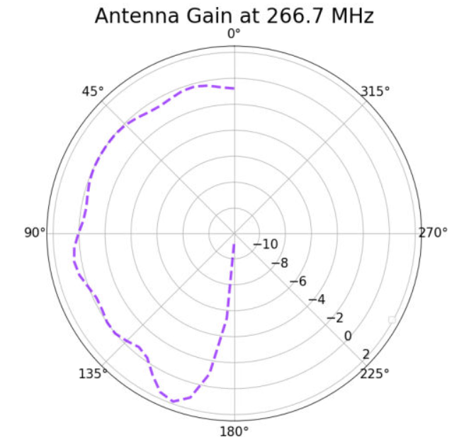
Also attached for reference are the gain pattern of the associated individual from the AREA output and the violin plot of the run producing the data. |
| Attachment 1: 20230410_AREA_PoR_CosTheta_bestIndiv_singleFreqTest.PNG
|  |
| Attachment 2: 20230201_singleFreqTest_100NPop_fitnessPlot_10Gens.PNG
|  |
| Attachment 3: 20230410_AREA_mostFitIndivReUpload_singleFreqTest.PNG
|  |
|
|
210
|
Wed Apr 5 17:21:07 2023 |
Nick King | H-pol XF Design | Work in progress. Update on H-pol XF design. The first plot is the gain pattern with ferrite rod sets (blue) vs. with nothing but the copper plates.
The second plot is the gain pattern with everything but the ferrite rod sets vs. with nothing but the copper plates.
The ferrite rod sets function to narrow the gain pattern. |
| Attachment 1: Screenshot_(7).png
| .png) |
| Attachment 2: Screenshot_(8).png
| .png) |
| Attachment 3: HpolfromScript(5_10_2023).png
| .png) |
| Attachment 4: StephHpolwith_just_copper_plates_and_wires.png
|  |
|
|
209
|
Tue Apr 4 13:51:56 2023 |
Alex M | Final To Do List for PUEO Loop | At the main GENETIS meeting yesterday, we collected the last few things that need to be worked out in order to get the PUEO loop in working order. Here's a list
-
Skeletonize the xmacros (Alex) 04/10/23 In progress
-
We need to modify PUEOsim to read in different gain files (Dylan) Changes made 04/10/23 Testing to be done.
-
Currently, PUEOsim reads in files like vv_0, vh_el, etc. It needs to be modified to take in the gainfiles as arguments and read different ones for each individual.
-
Requiers slight modification of the batch job scripts, but these are relatively small
-
Slight modification on the fitness score read in script (Dylan) Changes made 04/10/23 Testing to be done.
-
Fix Ezio's comments on XFintoPUEO.py and modify to read in outputs from two files (Jacob) 04/10/23 in progress, further work this week
-
Since we are running XF twice (once for each power source), we need the conversion script to read in from two files and print out to 8 files (vv_0, vh_el, etc)
|
|
|
208
|
Wed Mar 29 18:36:29 2023 |
Alex M | GENETIS Working Meeting Update | This is an entry for the usual Wednesday working meeting GENETIS holds. We are largely carrying on from last week's hackathon hammering out the remaining pieces that need to be fixed. See the previous ELOG post for a list of those.
Alex
Amy pointed out on the Monday call that the proper way to simulate the ANITA antenas is to use one source at a time. I modified the script I had so that it makes two simulations per antenna. The first one will use the power source connected to the "VPol" ridges and the second one uses the one connected to the "HPol" ridges. After checking this, it looks like the asymmetry I had pointed out before fell away. In other words, I think XF only wanted to use a single power source anyway. So now we should be able to produce the VV, HH, VH, and HV data that icemc and PUEOsim need.
Ryan and I also worked a bit on the slopes of the ridges. We experimented with the parameter that affects the curvature, which seems to be able to be too large. But many of the designs still look to have almost no slope and many still caved inward rather than sloping outward. We're still working on figuring out what causes that, but I think it means we need another constraint on distance of the top of the inner ridges from the center.
We also tried figuring out why the sides of the curved part of the ridges don't stay in the same plane as the straight part of the ridges. I'm confident that they do stay in a single plane (I attached a Mathematica notebook that shows as much by finding that the torsion of the curve is zero; for some reason I couldn't print it to a PDF). We think that we should be able to rotate the curve into the same plane as the straight part of the ridge, but I haven't figured out how yet.
Nick and I continued working on the HPol antenna. We want to check if there are any other things in Steph's example XF file that are significant to the results of the simulation (versus just being there as a representation of the model). It looks like there are, and Nick is working to figure out what they are by deleting them (in a copy) and generating simulation results for them to compare to the original. Otherwise, the most significant parts (the copper plates) are now being made in a script and just need to be connected to one another.
Dylan
I tried to build root from source again and ran into an error 3 hours into the build. I messaged Will and asked if he knew anything about the error. I then reran the build with Will's suggested change and ran into the same error 3 hours later. I did, however, manage to build pueo by sourcing the installation of root in Will's shared pueo directory. I'm now testing getting a txt output file from the simulation as it turns out my initial solution didn't work.
Update:
I got a working version of root installed. Also, I was able to modify pueoSim to output a veff.txt file. Now, I need to modify where it reads in the gain files, and then modify the icemc specific bash scripts to work for pueosim. |
| Attachment 1: Modeling_ANITA_Ridges.nb
|
(* Content-type: application/vnd.wolfram.mathematica *)

(*** Wolfram Notebook File ***)
(* http://www.wolfram.com/nb *)

(* CreatedBy='Mathematica 12.0' *)

(*CacheID: 234*)
(* Internal cache information:
NotebookFileLineBreakTest
NotebookFileLineBreakTest
NotebookDataPosition[       158,          7]
NotebookDataLength[    141335,       3108]
NotebookOptionsPosition[    137462,       3039]
NotebookOutlinePosition[    137824,       3055]
CellTagsIndexPosition[    137781,       3052]
WindowFrame->Normal*)

(* Beginning of Notebook Content *)
Notebook[{
Cell[BoxData[""], "Input",
 CellChangeTimes->{{3.889104537246646*^9, 3.8891045516248693`*^9}, {
   3.88910472825602*^9, 3.889104729415251*^9},
   3.889118788593347*^9},ExpressionUUID->"f2d7bf67-519b-4366-9a10-\
f19376de6bb8"],

Cell["<\
Here, I will use an example ridge that I have made and tested in XF to \
demonstrate how the curved part of the ridges slope in.
Here is a figure that represents one of these ridges. We are viewing it \
directly at the edge of the ridge, so the blue line actually represents the \
side. The purple curve should lie directly aligned with the blue line but \
doesn[CloseCurlyQuote]t. The same goes for the green line and orange/red \
lines (which do lie in the same plane, but that plane isn[CloseCurlyQuote]t \
aligned with the other side) below, which is the other side of the ridge.\
\>", "Text",
 CellChangeTimes->{{3.889118836397954*^9,
  3.889119017191614*^9}},ExpressionUUID->"0859e4b4-741b-4eea-b2b6-\
e446b9af7816"],

Cell[BoxData[
 RowBox[{
  RowBox[{"x0", "=", "4"}], ";", " ",
  RowBox[{"y0", "=", "4"}], ";",
  RowBox[{"z0", "=", "0"}], ";", " ",
  RowBox[{"yf", "=", "6"}], ";", " ",
  RowBox[{"H", "=", "30"}], ";", " ",
  RowBox[{"zf", "=", "30"}], ";", " ",
  RowBox[{"xf", "=", "zf"}], ";", " ",
  RowBox[{"[Beta]", "=", "2"}], ";",
  RowBox[{"[Tau]", "=", "0.26"}], ";"}]], "Input",
 CellChangeTimes->{{3.8891047313587914`*^9, 3.889104784350019*^9}, {
  3.889105008478373*^9, 3.889105011515078*^9}, {3.889106004732277*^9,
  3.88910602661027*^9}, {3.889112979624475*^9, 3.889112979661337*^9}, {
  3.8891130240801353`*^9, 3.889113037799301*^9}},
 CellLabel->
  "In[433]:=",ExpressionUUID->"fb3dee39-fae9-47d5-bb54-52d21df6980e"],

Cell[CellGroupData[{

Cell[BoxData[
 RowBox[{"ParametricPlot3D", "[",
  RowBox[{
   RowBox[{"{", "[IndentingNewLine]",
    RowBox[{
     RowBox[{"{",
      RowBox[{
       RowBox[{"x0", "+",
        RowBox[{
         RowBox[{
          RowBox[{"(",
           RowBox[{"zf", "-", "x0"}], ")"}], "/", "[Tau]"}], "*", "t"}]}],
       ",",
       RowBox[{"y0", "+",
        RowBox[{
         RowBox[{
          RowBox[{"(",
           RowBox[{"yf", "-", "y0"}], ")"}], "/", "[Tau]"}], "*", "t"}]}],
       ",",
       RowBox[{
        RowBox[{
         RowBox[{"(",
          RowBox[{"zf", "-", "z0"}], ")"}], "/", "[Tau]"}], "*", "t"}]}],
      "}"}], ",", "[IndentingNewLine]",
     RowBox[{"{",
      RowBox[{
       RowBox[{"x0", "+",
        RowBox[{
         RowBox[{
          RowBox[{"(",
           RowBox[{"zf", "-", "x0"}], ")"}], "/", "[Tau]"}], "*", "t"}]}],
       ",",
       RowBox[{
        RowBox[{"-", "y0"}], "-",
        RowBox[{
         RowBox[{
          RowBox[{"(",
           RowBox[{"yf", "-", "y0"}], ")"}], "/", "[Tau]"}], "*", "t"}]}],
       ",",
       RowBox[{
        RowBox[{
         RowBox[{"(",
          RowBox[{"zf", "-", "z0"}], ")"}], "/", "[Tau]"}], "*", "t"}]}],
      "}"}], ",", "[IndentingNewLine]",
     RowBox[{"{",
      RowBox[{
       RowBox[{"x0", "+",
        RowBox[{
         RowBox[{
          RowBox[{"(",
           RowBox[{"xf", "-", "x0"}], ")"}], "/", "[Tau]"}], "*", "t"}]}],
       ",", "y0", ",", "z0"}], "}"}], ",", "[IndentingNewLine]",
     RowBox[{"{",
      RowBox[{
       RowBox[{"x0", "+",
        RowBox[{
         RowBox[{
          RowBox[{"(",
           RowBox[{"xf", "-", "x0"}], ")"}], "/", "[Tau]"}], "*", "t"}]}],
       ",",
       RowBox[{"-", "y0"}], ",", "z0"}], "}"}], ",", "[IndentingNewLine]",
     RowBox[{"{",
      RowBox[{
       RowBox[{"xf", "+",
        RowBox[{
         RowBox[{"xf", "/", "[Tau]"}], "*", "t"}]}], ",", "yf", ",", "zf"}],
      "}"}], ",", "[IndentingNewLine]",
     RowBox[{"{",
      RowBox[{
       RowBox[{"xf", "+",
        RowBox[{
         RowBox[{"xf", "/", "[Tau]"}], "*", "t"}]}], ",",
       RowBox[{"-", "yf"}], ",", "zf"}], "}"}], ",", "[IndentingNewLine]",
     RowBox[{"{",
      RowBox[{
       RowBox[{"xf", "+",
        RowBox[{
         RowBox[{"zf", "/", "[Tau]"}], "*", "t"}]}], ",",
       RowBox[{"y0", "+",
        RowBox[{
         RowBox[{
          RowBox[{"(",
           RowBox[{"yf", "-", "y0"}], ")"}], "/", "[Tau]"}], "*", "t"}]}],
       ",",
       RowBox[{
        RowBox[{"zf", "/", "[Tau]"}], "*", "t"}]}], "}"}], ",",
     "[IndentingNewLine]",
     RowBox[{"{",
      RowBox[{
       RowBox[{"xf", "+",
        RowBox[{
         RowBox[{"zf", "/", "[Tau]"}], "*", "t"}]}], ",",
       RowBox[{
        RowBox[{"-", "y0"}], "-",
        RowBox[{
         RowBox[{
          RowBox[{"(",
           RowBox[{"yf", "-", "y0"}], ")"}], "/", "[Tau]"}], "*", "t"}]}],
       ",",
       RowBox[{
        RowBox[{"zf", "/", "[Tau]"}], "*", "t"}]}], "}"}], ",",
     "[IndentingNewLine]",
     RowBox[{"{",
      RowBox[{
       RowBox[{"x0", "+",
        RowBox[{
         RowBox[{
          RowBox[{"(",
           RowBox[{"zf", "-", "x0"}], ")"}], "/", "[Tau]"}], "*", "t"}]}],
       ",",
       RowBox[{"y0", "+",
        RowBox[{
         RowBox[{
          RowBox[{"(",
           RowBox[{"yf", "-", "y0"}], ")"}], "/", "[Tau]"}], "*", "t"}]}],
       ",",
       RowBox[{"[Beta]", "*",
        RowBox[{"Log", "[",
         RowBox[{
          RowBox[{
           RowBox[{"t", "/", "[Tau]"}], "*",
           RowBox[{"(",
            RowBox[{
             RowBox[{"Exp", "[",
              RowBox[{"zf", "/", "[Beta]"}], "]"}], "-", "1"}], ")"}]}], "+",
           "1"}], "]"}]}]}], "}"}], ",", "[IndentingNewLine]",
     RowBox[{"{",
      RowBox[{
       RowBox[{"x0", "+",
        RowBox[{
         RowBox[{
          RowBox[{"(",
           RowBox[{"zf", "-", "x0"}], ")"}], "/", "[Tau]"}], "*", "t"}]}],
       ",",
       RowBox[{
        RowBox[{"-", "y0"}], "-",
        RowBox[{
         RowBox[{
          RowBox[{"(",
           RowBox[{"yf", "-", "y0"}], ")"}], "/", "[Tau]"}], "*", "t"}]}],
       ",",
       RowBox[{"[Beta]", "*",
        RowBox[{"Log", "[",
         RowBox[{
          RowBox[{
           RowBox[{"t", "/", "[Tau]"}], "*",
           RowBox[{"(",
            RowBox[{
             RowBox[{"Exp", "[",
              RowBox[{"zf", "/", "[Beta]"}], "]"}], "-", "1"}], ")"}]}], "+",
           "1"}], "]"}]}]}], "}"}]}], "[IndentingNewLine]", "}"}], ",",
   RowBox[{"{",
    RowBox[{"t", ",", "0", ",", "[Tau]"}], "}"}]}], "]"}]], "Input",
 CellChangeTimes->{{3.889104789299713*^9, 3.889105080982005*^9}, {
   3.88910513362922*^9, 3.889105134787335*^9}, {3.889105176753415*^9,
   3.889105183526766*^9}, {3.889105234070648*^9, 3.8891053106544733`*^9}, {
   3.8891053894877863`*^9, 3.889105467143161*^9}, {3.889105814148295*^9,
   3.889105946276293*^9}, 3.88911016079349*^9, 3.889111844551866*^9},
 CellLabel->
  "In[434]:=",ExpressionUUID->"a2747aaf-59c9-498b-a918-186b6556d2ae"],

Cell[BoxData[
 Graphics3DBox[{{{}, {},
    TagBox[
     {RGBColor[0.368417, 0.506779, 0.709798], AbsoluteThickness[2],
      Line3DBox[CompressedData["
1:eJwVjHk41Isexh1ahha/2fyQiIZkG2Mf/JrXcitCi4RzSUI8t1G3EUqbJCod
RyqpQ9f2KGSo64QkmpTUTWWP0mI5kVD2/c75432+z/t5Pu9Xc+/BHUGyMjIy
rtLISePx7o+1MjIEVK0qZf++4511NZyEnA0FF57G6NEINETP1GdIedNN5aN2
bTGCX2yHPu8kCFyo4/9h9wsBsF/vVW5LFohv2mfkrSEw/et90zOyBCK25bfK
tWUJlgT2qbnbEXh3oihwyWIC9EEyear1nqB00EIpN4ZA6pPMZ8sVCHx86HZw
tFUiUFnUQHNZTIfS1rgLKiwCGzn9H360Ngg+GNEGrykwQN+3lWGqS2Cq1fLq
cOsXgc6zO10cOxaCzj6S1LoTkDjcynmbNSKoD35xUmeHEmaXilYfPU5g1cfy
3r0Gc4KJNxkptV7KOC/apLE7hwBT6Je/1EEOn44VvfNNUMXh+qnHOa8JJPE2
Vrh50KDHs5SEpKoh87fhlbRJAq2pxtU/iBUw051oDnmrDv0NNbP/W0tHQs6p
17IqdPiNWJouil6DOy3ll5660UFe6Tp/OZ2JplZjt8RYTRxsGHnTHkFH/E6n
DQ3jbOh9eDrP+I8WkqoU7m7PoiOMn+lXF6MMcTAp25C7FqOK+2x6XtDhODQd
daBLFaMeT5/syePAdXOX8M5POmJst/urWq2GapDiqv7H2lgkogTNqxmwEV8v
OVmlgQNT7KeFtTqYm++oUN3IgHDyR/TzFZrIEZctEnatw84Tnu8eH2JgUp/o
NPTQwvXaUtnpKV1kdo2mp6UxYF1wJyMlZS0eBYW5S+bWg1fYsvxKDQNDDOc9
uyQc1HBe8s+S+lAPuar2fYiBLxf37BIt1cFUyEdRjLoB3OJSW/YqM7FpKNKp
x2IdiPrf7aJsDNFx9QjP2pGJbwG0sJJTuuhNSau3czfC7t+iTP9xkAlHDikb
L1mPge4gsYMXF5yv1R+F15ggXukkFg/poS+vh57BN8Zms26DcQkTq84VbbOw
MMBo9nh4RaUxxF1bOGnfmLimzyeYwYb49Nq8fIOAB4VjzZJwJgsvVO3MRy4Z
wXa5w6aqlzzUyNnK3t3AgrWaJInbwgU3QTz/3s0E1UO932jBLCjKZR32jzFG
supXmcn3JlB9dSBCksyCxmkNW28dHlo6tn6JCjHFv5KVbxdVsrBc2+f+jloe
/vuR/f1GvylmHyyJLe9hgUepFEX6mmBhJM++LNIMA01vZbTpbIR3Mp44y5ii
yzntsWjGDOo7Pq8r5LPxc+Sih1OqKW41PtS4etwcm0oZ4yH+bDhzn91wMjRD
h7DgeQnNAq9WaAbFXWRDMmIzM1FvhlubJ28cSrBASm3YyeoSNkQGJu1vg8zR
ZcYs01exxENRtpXPJzbsBwObvOUtUBZwcT4m3RLap8l0lrwSnDnKriuyLCCs
MeXYa1ghNrLwtgxPCUbRF45ILC2RZJ53Zb7ACvBb4+HmowTjIH6VdrslXPqO
G3lx+RDktxaUxSpB+CgktuSQFY4WqjOLKvlI692fHVushNqMpsAfbD7isgdb
Qp2sMaigZR/boYS52wsT3FI+9N6r1dS9tMaZZLWEDDkSQu0C+Ruu1hBoq8xq
edsgYtnoYXUuiRm9yxb3hq0xUBzmq/LBBgV/KcqXe5KQ5Mx8HjtngyMHZtMj
d9uipcDVMf4UiUDHtbBRt0W4rfv6xn5b+PmHrCnNJ6EdGl9uVG0LeVda58tQ
CnpRtblyjSQ0FIR3XT0pzP0uFLP+TWFvsGZqqZSLHU5EDXtTGGx4c9JXRCF1
57Hz+5tI2JxIdLjsQ6HR67rGUASFJVyusLGZhOdwcXObP4X0QD1/RjSFL10p
vOw2EoktY1MBQgq84y7dXskUrrvue2jfSWI+65R91GkKvxYk9ffcp0DTXNxw
uo9Ep83lxtwCCi6Dow+MyikIVvo9Me8nsT88J81JLO0874TICgoRM2UlfVI+
Lf4zaKCYgnappoF8NYXuZuG17QMklLXaJnjSv0OSe6EGdRSqLzT5aA6R2Epb
rVYp9c60Nw2LOihEjmb/VT1KoqopN7CxWfp3Nf9xxQcK4s9zbYfHSLitLDOM
aKMQsif90qJPFHrqPV/ojpPo2FQ3rizdu/YGmaR0U3DPW1aYNEFi4sG3c7ul
HvlzPKz8OwWj3WGiPdMkjDKNC/v6KSiY/9NRdpjCvi2vAlgzJCrb7SIuSr3Z
yCrWlp8U0qzWeTyXcmeWu4Ar9T7Pxf/5fly6Y3ZYGs+R2Bcf/vbwGIUmDJzV
nqJgJ2O+vlvKx6rjbpCTFJ6d2bbrwAyFI98TVVPnScRMXwt4ME2h9FmJTukc
haL2r8tcFkgomuUZ+Ep7vrzKxMIChd5a+7kFKb8Z+mDs7/5/SZ4y2A==
       "]]},
     Annotation[#, "Charting`Private`Tag$112685#1"]& ],
    TagBox[
     {RGBColor[0.880722, 0.611041, 0.142051], AbsoluteThickness[2],
      Line3DBox[CompressedData["
1:eJwVjHk81Psexh1UQ4vfbH7IEs1ItjH2YX7Nx3IrQouEc0mWKa/bpNvYSpsk
CseRCjl0bS8lGdV1siXfJpG6qewRkuVEQtmX4c754/njeb/ez6MdcPIAX1ZG
RsZVGjlpPD7+sVVGBgM16xopxtBsb2MdI7FgR3HCyxh9EgbN0UtNOVLeekfl
jF1nDO8X7kT/QQyDhEbOH3a/YAjo7wJUOlN5ojv2OUVbMFj89YnZZVkMRey7
3yHXmcdbGzSi7m6HwcfzpUFr12CIPI6nLnQ85pWPWyoXxmCQ8SK3foMihvqe
up2c7hDzVOWbSS5ryKC8Ny5BlYahnYzRnh8dzbweY9J4uiIFyEf3Usz0MLTQ
YXVrsuMLT7f+wQDDjgb8K8/EDe4YEjvcLfiQN8VrOvb6gu4BZVheJ9Q4cw5D
m/sqhwMMJby59zlpDV4qcE24S+twAYaoAr/76xzk4PPZ0o++iWoQ1rTwvOAd
hlLYO6vdPEigz7YSB2eoQ+5vk5tI8xjqyDBBP7CNYK431xb8QRMMdtQt/28r
GSUWXHwnq0oGvykrM/noLfCgvfL6Szcywm8OXLuRTYXWDhO35FhtONk89b4r
goziDzrtaJ6lg37PyxXKf3QgpVbx0f48Mgrl5Po1xqiA6Bgu21y4FaaVjtoO
vSYjx4nFqJABNZj2ePniSBEDXHcPCB78JKMY7n5/NWsNUOMrbR59zgR5IcFr
06AgW9Htsgu1WhCyQH9Z0qALkpXuarWdFCSY/xH9aqM2FIgq5AUD2+Dgec+P
z09R0LwB1mvkoQO3G8plFxf0IHdgOjsri4Jsih/kpKVthWf8UHexZDuwS9o3
3KyjoAmK85FDYgbUMd5wruAGoBl8S/37BAV9STpySLhOFxaC+4QxmobgFpfR
HqBCRbsmIp2GLLcB1vS7XZStEXTfOs22caSib4Gk0LKLejCcltVk524Mh3+L
MvvHSSpyZOCy8eLtMDbIFzl4sYDxFfUJ0qkIe6ub/HBCH0aKhsg5HBPYbT5o
OCumos1XS/dZWhrCdP5seHWNCYgG9jCyvlFRugEHox4zgs/vLCp38NigeLZN
HE6loddqdhZT142Bu8FhV+0bNtTJcWUf7aAhG3VxCqudBaxE0conN1NAE8Pf
SMdoSEkuL8w/xgRS1b7KzH8yBbW3IRHiVBrSuqTF9dZlQ3v33i9RwWbwr1SV
e6U1NLSB6fPkQAMb/ttH/545agbLVWtjK4doiE2olkb6msLqVJF9RaQ5jLV+
kGGS6Si8l/LCWcYMBpyznguXzEHzQP+2Eg4d/ZxK8nDKMIO7LU+1bp2zgF3l
lNlgfzpyZtVnOhmZQ7eg+FUZyRLebtTmxyXRkXjKdmmuyRzu7p7PPJVoCWkN
oRdQGR0JDU27PvAtYMCcWmGgagVPhfnWPp/pyH48qNVbwRIqApNWYrKtgHkJ
z6YpKCNnhorrxjxLENSZMey1rCE2suSeDFsZGUcnnBZbWUGKRdHNlWJrAL8t
Hm4+ysiEz6lldlmBy8g5Yy8WB3j3O4orYpWR4FlwbNkpazhTokktreFA1vDx
/NiHyqghpzXoB50Dcfnj7SecbGBcUcc+tlsZSe6tzrHKOaD/Sb2u8Y0NXE5V
T8yRw5GAWayQ6WoDPKbqso63LUSsnw7TZOFoSf+G5eNJGxh7GOqr2mMLxX8p
KVR64khcsNQ/c9UWTocsZ0ce5kJ7satj/EUcBTluBVtNLoRz3be3jHLBzz94
... 2817 more lines ...
|
|
|
207
|
Mon Mar 27 13:10:02 2023 |
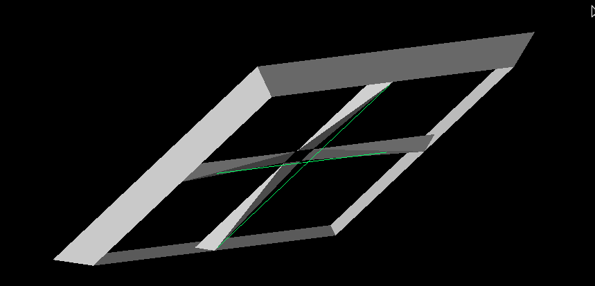
Alex M | GENETIS Hackathon Summary and Next Steps | This entry will serve to summarize what tasks we've completed and still need to complete after last week's GENETIS hackathon.
Alex
My focus was on the XF scripting for making the PUEO antenna. Before last week, we had a script which made the geometry of a PUEO-like antenna. The xmacro script has been modified in the following ways:
- Now includes power sources connecting the ridges that are opposite each other.
- Generalized to use variables without hardcoding.
- Reads in data from the output files of the PUEO GA.
- Loops over all read in antennas to set up all of the simulations at once.
At this point, the script for setting up the simulations of the PUEO loop is just about ready for use. The only change to be made is to the frequency list. The script for printing out the gain data is also ready, though it only prints out the gain in theta and phi, not the cross polarization.
Here are some outstanding points that need to be hammered out, though they impede the quality and accuracy of a run rather than the actual functioning of the loop.
- The shape of the ridges in the generated antennas from the GA are considerably different from the PUEO antenna.
- This is likely something that can be fixed by adjusting the constraints--the subspace of the parameter space that leads to PUEO-like ridges may be very small as-is.
- You can see an example of an antenna from the GA attached (viewed from slightly below). It looks dramatically different. This seems to be due to constraints on the height and width being too small, but the ridges are also clearly misshapen.
- The curve on the ridges looks like it needs some work.
- For very PUEO-like antennas, the slopes look reasonable, but they do flare in or out slightly. This is more dramatic for ridges that deviate from PUEO's significantly.
- My best guess is that the parametric form of the curves is placing the curves in a plane that is different from the rest of the ridge. This should be fixable by somehow constraining the curve to a given plane.
- The simulation still only outputs polarization data for theta and phi, not the cross polarization.
- It looks like XF naturally gives us the theta and phi polarization. It's not clear how to get the cross polarization gain (which we think means the gain when the signal is at 45 degrees).
- One idea is to redo the simulation but with the antenna rotated 45 degrees in the azimuth. But I'm not certain that that iwll work.
- Amy indicated that the correct way to do this is by simulating the antenna with just one power source at a time.
- Leaving the VPol source would produce the VV and VH data and leaving the HPol would produce the HH and HV data (HV and VH could be flipped!).
- Currently, the antennas have a fixed opening angle. We'd like to add this as a parameter, though at the moment it might be ok to forego that.
- We need to make sure that the power sources aren't too close together (fixed!).
To do for this week:
1. Modify the script to make two simulations for each antenna, each with only one power source.
2. Adjust the constriants on the parameters to fix the curvature.
3. When we begin a run, we will want to just evolve the height and the inner side length (these determine both the inner side length and the outer side length).
Dylan and Jacob
Dylan and Jacob focused on getting PUEOsim/icemc working, which will be the simulation software needed for the PUEO loop. Here's a summary from Dylan:
- Plotting and bash scripts should be mostly good to go.
- Currently have 4/5 of the PUEO prerequisites for pueoBuilder, and the GENETIS-specific code is ready to implement and test when it's built. I’m trying to build the correct root version one more time before today’s meeting, and if it fails again I’m going to ask Will.
- The main thing left is to get the correct version of root installed, which while annoying, shouldn't take too long
To do for this week:
1. Once PUEOsim is working, run it with the usual settings to get the default performance. It will need to be submitted as a job array (ask Alex for help with this if you need; ask Will for advice on how many neutrinos to run).
|
| Attachment 1: Weird_PUEO_Model.png
|  |
|
|
206
|
Tue Mar 21 17:58:21 2023 |
Alex M | GENETIS Hackathon Day 2 | Today was day two of the GENETIS hackathon. See the previous entry for details on day one.
Alex
I continued working on the XF scripting for the PUEO horn antenna. Amy showed me an actual horn antenna from ANITA in Lisa's office so I could get the dimensions and see how the loads (power sources in XF) were offset. Offsetting the power sources led to fixing the asyemmtry problem from yesterday. I tested offsetting the loads by various heights and found that they all give the same gain patterns except for when they overlap, proving that they were interfering with each other when they crossed.
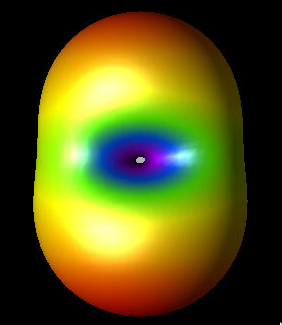
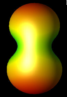
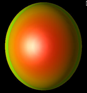
There is still, however, an asymmetry between the x and y axes (but the gain patterns are now symmetric across either of them). This is more reasonable, though I'm not positive that it should be this way. I attached an image of the gain pattern to show this asymmetry. Note that it is still at 83 MHz, which is well outside the PUEO bandwidth, but higher frequency gain patterns show the same thing (but they have more nodes so they're harder to look at). I attached images from the x-axis, y-axis, and above of the gain pattern. One way to check this will be to compare to the data stored in PUEOsim/icemc and see if they demonstrate similar asymmetries.
My next step is to test the constraints we've decided on using the script. I'll try out a few different values of the parameters and then if everything is working I'll use the GA Ryan and Dylan wrote to generate many individuals and have XF make the models for them. We don't necessarily need to see the simulation outputs from those XF runs, we just need to see if we run into error. Beyond that, we need to figure out how to extract the proper gain data from XF to create the same format that PUEOsim and icemc use.
Amy also mentioned that we should add the opening angle of the horn antenna as a gene. This may be a little tricky but should be doable. Once we are set with the current XF script and changing the data formatting to match what PUEOsim and icemc need, I'll work on adding that as a gene.
Dylan and Jacob
We tried to get IceMC running and able to read in gain files - we failed. Something was wrong with my make files and Jacob’s c++ compiler, so neither of us got a working version of IceMC. We then switched gears to focus on pueoSim. I created a branch on the nicemc github to output a veff.txt in the format of IceMC, so we can reuse the already-made code. Jacob and I also have been trying to install pueoSim, but we’ve been running into many errors and issues from the “C++ Gods”. For the next steps, I will finish the veffective branch and create a pull request. Then, I will work on a branch to make it so pueoSim can read in a variable path to the gain files.
Ryan
Tuesday: Created a new branch on the PEUO repository, version0.0, and placed the repository in the same location as the Ara one for familiarity. I also added an alias to this directory onto the genstudents channel if people would like to add the path to their .bashrc's. I then went through the the Evolutionary_Loop directory and cleaned up any residual Ara based files that were not needed to run this loop. This will make navigating and troubleshooting easier as we finish building. This branch was then commited and pushed to the github and submitted a pull request. |
| Attachment 1: ANITA_Gain_X.png
|  |
| Attachment 2: ANITA_Gain_Y.png
|  |
| Attachment 3: ANITA_Gain_Z.png
|  |
| Attachment 4: Top_Down_ANITA.png
| 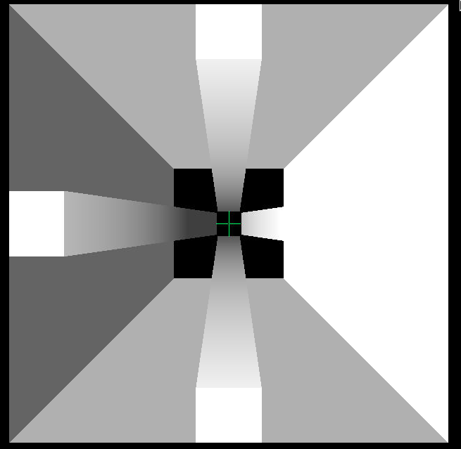 |
|
|
205
|
Mon Mar 20 17:32:42 2023 |
Alex M | GENETIS Hackathon Day 1 | Today was the first day of the GENETIS Hackathon. We are spending several days this week specifically tackling the PUEO project to get it into full form (or close to it). Here is a progress update after day 1.
Alex
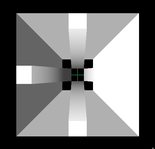
I am working on the xmacro script for the ANITA antenna. Before today, we had a working xmacro script to make the geometry of the ANITA horn antenna. Now I am trying to modify it to make it 1) more true to the actual ANITA antenna (in terms of which parts are electrically connected) and 2) add in the power source and sensors so that we can get simulation results. I've attached the xmacro script here along with a picture of the geometry and some gain patterns. There are four ridges in the antenna. They are all connected by the outer walls of the antenna. However, only the ones directly across from each other are connected by a load (in this case, a power source, since we simulate as a radiator). So we have two power sources, one connected each "ridge bicone".
In making this, I have generated some gain patterns. I want to test a few cases to see if the results coming from XF seem reasonable, though I don't know what I should expect the gain pattern to look like when I've done things correctly. Here are the options I'll compare:
- Just use one "ridge bicone".
- Use two "ridge bicones" with the walls but just one power source.
- Use two "ridge bicones" without the walls and two power sources.
- Use the full form, with two "ridge bicones", walls, and two power sources.
Case (4) is the one I expect to be correct. However, when I simulate that, I get a slightly asymmetric gain pattern compared to what I expect (I expect symmetry across the "ridge bicones"). You can see from the attached image that there is a strange preference in one corner. My guess is that this has to do with which ridges are set to be ground and which are set to 1V (the potential). Feel free to ask me for more details about these figures/scripts on slack and I'll fill them in on here. I'll clean up the script and add in full test cases later this week.
The image of the antenna I attached is a bird's eye view. The green lines represent the power sources I've connected between the ridges. They do appear to overlap, but my understanding is that they are not actually affecting each other (they should just be a representation of the power sources).
The image of a gain pattern (which is 3D and also a bird's eye view) is for the case of the antenna with both power sources and the walls remaining (the antenna is still shown too, to demonstrate the asymmetry of the gain pattern). This is well outside of the frequency range ANITA cares about (83 MHz), and I haven't looked closely at the higher frequencies yet, but I still am surprised by the asymmetry. I'll update tomorrow with more gain patterns to compare.
Dylan and Jacob
Dylan and Jacob are working on the bash scripts for the PUEO loop. They are taking the parts of the bicone loop that are specific to ARA/bicones and changing them to be specific to the PUEO loop.
All the bash scripting outside of implementing the new software we’re developing should now be complete (we just need to debug when we do test runs). The new GA is implemented into the PUEO loop. We tried and failed to build a version of pueoSim on our own. Will has provided us with a precompiled version and instructions for installing it on our users as well as access to the necessary pueoBuilder repo. Jacob and Dylan are scheduled to go through the installation with him on Thursday at 4pm in his office, M2024.
We have also found that peuoSim currently only outputs root files. So, we will need to create a conversion script or modify pueoSim for when we implement it into the loop. Currently, using IceMC looks to be the easiest way to get a test run going. For the next steps, we have a plan for making IceMC read in a variable file path name to avoid recompiles and issues with parallelization (Alex has given us the path to look at how ARA does it). Then, we will work on installing pueoSim and testing its current viability.
Bryan
Upon checking the existing plotting scripts used for previous GENETIS work, it appears that they can be used for PUEO with minimal changes. In order to test the plotting scripts, sample output data from the PUEO loop is needed, or at least test data that mimics the form of the output for the PUEO loop. After more progress is made with installing an MC package and the PUEO loop can be run to produce test outputs, the plotting scripts can be tested and implemented in the bash script. |
| Attachment 1: ANITA_Antenna_Project.xmacro
|
App.getActiveProject().getGeometryAssembly().clear();
var freq = [83.33, 100.00, 116.67, 133.33, 150.00, 166.67, 183.34, 200.00, 216.67, 233.34, 250.00, 266.67, 283.34, 300.00, 316.67, 333.34, 350.00, 366.67, 383.34, 400.01, 416.67, 433.34, 450.01, 466.67, 483.34, 500.01, 516.68, 533.34, 550.01, 566.68, 583.34, 600.01, 616.68, 633.34, 650.01, 666.68, 683.35, 700.01, 716.68, 733.35, 750.01, 766.68, 783.35, 800.01, 816.68, 833.35, 850.02, 866.68, 883.35, 900.02, 916.68, 933.35, 950.02, 966.68, 983.35, 1000.00, 1016.70, 1033.40, 1050.00, 1066.70]
CreatePEC();
var units = " cm";
num_ridges = 4; // either 2 or 4
// Make the walls and a ridge
build_walls(10,1,30);
// Note that to avoid overlap, we need x0 >= y0
x0=0.04001; // previously 0.04
y0=0.04; // previously 0.04
build_ridges(x0, y0, 0.0, 0.1, 0.06, 0.3, 0.26, 0.1, 0.1, 1);
CreateAntennaSource();
CreateGrid();
CreateSensors();
CreateAntennaSimulationData();
QueueSimulation();

// Try making copies of the ridge
var new_ridges = new EllipticalPattern();
Output.println(new_ridges.getInstances());
new_ridges.setInstances(7);
//new_ridges.clone();
//Output.println(new_ridges);

// Makes the outer walls of the horn antenna
// S is the side length of the bottom of the wall
// a is the coefficient for the linear function the walls extrude according to
function build_walls(S,m,H)
{
	// Make the edges to define the square
	var edge1 = Line( new Cartesian3D(-S + units,-S + units, 0), new Cartesian3D(-S + units, S + units, 0));
	var edge2 = Line( new Cartesian3D(-S + units, S + units, 0), new Cartesian3D(S + units, S + units, 0));
	var edge3 = Line( new Cartesian3D(S + units,S + units, 0), new Cartesian3D(S + units, -S + units, 0));
	var edge4 = Line( new Cartesian3D(S + units,-S + units, 0), new Cartesian3D(-S + units, -S + units, 0));

	// Declare sketches to be made from the edges
	var wallSegment = new Sketch();
	var bottomSegment = new Sketch();
	wallSegment.addEdge(edge1);
	wallSegment.addEdge(edge2);
	wallSegment.addEdge(edge3);
	wallSegment.addEdge(edge4);
	bottomSegment.addEdge(edge1);
	bottomSegment.addEdge(edge2);
	bottomSegment.addEdge(edge3);
	bottomSegment.addEdge(edge4);

	// Let's start by making the bottom
	var bottomCover = new Cover(bottomSegment);
	var bottomRecipe = new Recipe();
	bottomRecipe.append( bottomCover );
	var bottomModel = new Model();
	bottomModel.setRecipe( bottomRecipe );
	// Add the surface
	//var bottom = App.getActiveProject().getGeometryAssembly().append(bottomModel);
	//bottom.name = "Bottom square";

	// Now we need to extrude the edges to get height
	var walls = new Extrude( wallSegment, H + units);				// Makes an Extrude
	var wallOptions = walls.getOptions();						// Gives the possible options for
	// We will use the draft law option to extrude linearly
	wallOptions.draftOption = SweepOptions.DraftLaw;			// allows for draftlaw
	wallOptions.draftLaw = "("+m+"*x)";							// Set the expression for the extrude
	wallOptions.draftOption = 4;								// 4 indicates we use draftlaw
    //Walter - Change the gap type to Extended to get the desired shape
	wallOptions.gapType = SweepOptions.Extended; 				// I actually don't like this when we have x^2, but it doesn't do much for just x
    //Walter - Create a shell instead of a solid part
	wallOptions.createSolid = false;							// This way the shape isn't filled in
	walls.setOptions ( wallOptions );							// Sets the settings we assigned above

	// Make a recipe for a model
	var wallRecipe = new Recipe();
	wallRecipe.append(walls);
	var wallModel = new Model();
	wallModel.setRecipe(wallRecipe);
	wallModel.name = "Outer Walls";
	wallModel.getCoordinateSystem().translate(new Cartesian3D(0,0,0));	// Makes the model start at the origin

	// Set the material for these parts
	var wallProject = App.getActiveProject().getGeometryAssembly().append(wallModel);	// Adds the model to the project
	var pecMaterial = App.getActiveProject().getMaterialList().getMaterial( "PEC" );	// Makes the material available
	App.getActiveProject().setMaterial( wallProject, pecMaterial );						// Sets the material
	//App.getActiveProject().setMaterial( bottom, pecMaterial );						// Sets the material

}

// A function to build the inner ridges
// Here are the arguments, which are primarily used when making the LawEdges
// Bottom x distance from center
// Bottom y distance from center
// Top x distance from center
// Top y distance from center
// Full x
// Full y
// Full height
function build_ridges(x_0, y_0, z_0, x_f, y_f, z_f, tau, beta, S, m)
{

//	build_ridges(0.04, 0.04, 0.0, 0.1, 0.06, 0.3, 0.26, 0.1, 0.1, 1);

	// Logarithmic slopes
	//var Log1 = new LawEdge( "0.04 + u", "0.04 + 0.02/0.26*u", "1/10*ln((exp(3)-1.0)/0.26*u+1.0)", 0, 0.26); // alpha = z_max/beta
	//var Log2 = new LawEdge( "0.04 + u", "-0.04 - 0.02/0.26*u", "1/10*ln((exp(3)-1.0)/0.26*u+1.0)", 0, 0.26);

	var Log1 = new LawEdge( ""+x_0+" + ("+z_f+"-"+x_0+")/"+tau+"*u", ""+y_0+" + ("+y_f+"-"+y_0+")/"+tau+"*u", ""+beta+"*ln((exp("+z_f+"/"+beta+")-1.0)/"+tau+"*u+1.0)", 0, tau); // alpha = z_max/beta
	var Log2 = new LawEdge( ""+x_0+" + ("+z_f+"-"+x_0+")/"+tau+"*u", "-"+y_0+" - ("+y_f+"-"+y_0+")/"+tau+"*u", ""+beta+"*ln((exp("+z_f+"/"+beta+")-1.0)/"+tau+"*u+1.0)", 0, tau);


	// Inner straight slopes
	var IS1 = new LawEdge( ""+x_0+" + ("+z_f+"-"+x_0+")/"+tau+"*u", ""+y_0+" + ("+y_f+"-"+y_0+")/"+tau+"*u", "("+z_f+"-"+z_0+")/"+tau+"*u", 0, tau); // a_0 + at, b_0 + bt, c_0 + ct
	var IS2 = new LawEdge( ""+x_0+" + ("+z_f+"-"+x_0+")/"+tau+"*u", "-"+y_0+" - ("+y_f+"-"+y_0+")/"+tau+"*u", "("+z_f+"-"+z_0+")/"+tau+"*u", 0, tau);

	// Bottom line
	var BL1 = new LawEdge(""+x_0+" + ("+x_f+"-"+x_0+")/"+tau+"*u", ""+y_0+"", ""+z_0+"", 0, tau);
	var BL2 = new LawEdge(""+x_0+" + ("+x_f+"-"+x_0+")/"+tau+"*u", "-"+y_0+"", ""+z_0+"", 0, tau);

	// Top line
	var TL1 = new LawEdge(""+z_f+" + "+x_f+"/"+tau+"*u", ""+y_f+"", ""+z_f+"", 0, tau);
	var TL2 = new LawEdge(""+z_f+" + "+x_f+"/"+tau+"*u", "-"+y_f+"", ""+z_f+"", 0, tau);

	// Outer Straight slopes
	var OS1 = new LawEdge( ""+x_f+" + "+z_f+"/"+tau+"*u", ""+y_0+" + ("+y_f+" - "+y_0+")/"+tau+"*u", ""+z_f+"/"+tau+"*u", 0, tau);
	var OS2 = new LawEdge( ""+x_f+" + "+z_f+"/"+tau+"*u", "-"+y_0+" - ("+y_f+" - "+y_0+")/"+tau+"*u", ""+z_f+"/"+tau+"*u", 0, tau);

	// Inner top line
	var ITL = new LawEdge( ""+z_f+"", "-"+y_f+" + 2*"+y_f+"/"+tau+"*u", ""+z_f+"", 0, tau);

	// Outer top line
	var OTL = new LawEdge( ""+x_f+" + "+z_f+"", "-"+y_f+" + 2*"+y_f+"/"+tau+"*u", ""+z_f+"", 0, tau);

	// Inner bottom line
	var IBL = new LawEdge( ""+x_0+"", "-"+y_0+" + 2*"+y_0+"/"+tau+"*u", ""+z_0+"", 0, tau);

	// Outer bottom line
	var OBL = new LawEdge( ""+x_f+"", "-"+y_0+" + 2*"+y_0+"/"+tau+"*u", ""+z_0+"", 0, tau);

	// Make the sketches
	var straightEdge1 = new Sketch(); 	// All straight edges (IS1, BL1, TL1, OS1)
	var straightEdge2 = new Sketch(); 	// All straight edges (IS2, BL2, TL2, OS2)
	var curvedLog1 = new Sketch(); 		// Logarithmic edge (IS1 and Log1)
	var curvedLog2 = new Sketch(); 		// Logarithmic edge (IS2 and Log2)
	var topRectangle = new Sketch(); 	// Top rectangle
	var bottomRectangle = new Sketch(); // Bottom rectangle

	// Add the edges to the sketches
	straightEdge1.addEdges( [IS1, BL1, TL1, OS1] );	// Inner straight slope
	curvedLog1.addEdges( [IS1, Log1] );				// Right logarithm part
	straightEdge2.addEdges( [IS2, BL2, TL2, OS2] ); 	// Inner straight slope
	curvedLog2.addEdges( [IS2, Log2] );			 	// Left logarithm part
	topRectangle.addEdges( [ITL, OTL, TL1, TL2] );		// Top rectangle
	bottomRectangle.addEdges( [IBL, OBL, BL1, BL2] );	// Bottom Rectangle

	//WALTER - The Elliptical pattern is added as a recipe to the parts
	//In this case the location of the center and direction of the normal are simple, but for more complex scenarios, may need to use mroe functionality to find them.
	var ePattern = new EllipticalPattern();
	ePattern.setCenter(new CoordinateSystemPosition(0,0,0));
	ePattern.setNormal(new CoordinateSystemDirection(0,0,1));
	ePattern.setInstances(num_ridges);
	ePattern.setRotated(true);

	var cov = new Array();
	cov.push(new Cover(straightEdge1));
	cov.push(new Cover(straightEdge2));
	cov.push(new Cover(curvedLog1));
	cov.push(new Cover(curvedLog2));
	cov.push(new Cover(topRectangle));
	cov.push(new Cover(bottomRectangle));

	var pecMaterial = App.getActiveProject().getMaterialList().getMaterial( "PEC" );

	//WALTER - We can loop over all our parts and add them to the project as follows.  You can use similar concepts above.
	models = new Assembly();
	for(var w = 0; w < cov.length; w++)
	{
		var r = new Recipe();
		r.append(cov[w]);
		r.append(ePattern);
		var m = new Model();
		m.setRecipe(r);
		m.name = "Test Surface " + (w+1);
		//WALTER - Seperate array for the models, though we could just get them from the GemoetryAssembly again
		models.append(m);
		App.getActiveProject().setMaterial( m, pecMaterial );

	}

	// Work on the loft
	var vertex_position1 = curvedLog1.getPosition(curvedLog1.getVertexIds()[0]);
	var vertex_position2 = curvedLog2.getPosition(curvedLog2.getVertexIds()[0]);

	var loft = new Loft(models.at(2).pickFace(new Cartesian3D (0, 0, 0), vertex_position1, 0.5), "0.0", models.at(3).pickFace(new Cartesian3D(0,0,0), vertex_position2, 0.5), "0.0");
	loft.setPart1(models.at(2));
	loft.setPart2(models.at(3));

	var r12 = new Recipe();
	r12.append( loft );
	r12.append(ePattern);
	var m12 = new Model();
	m12.setRecipe( r12 );
	m12.name = "Loft 1";
	models.append(m12);

	//WALTER - append the assembly to the project, then loop over it to assign the material
	var assembly = App.getActiveProject().getGeometryAssembly().append(models);
	for(x = 0; x < assembly.size(); x++)
	{
		Output.println(assembly.at(x));
		App.getActiveProject().setMaterial( assembly.at(x), pecMaterial );
	}

}


// CreatPEC Function
function CreatePEC() //borrowed from XF demo
{
    //Make the material.  We will use PEC, or Perfect Electrical Conductor:
    var pec = new Material();
    pec.name = "PEC";
    var pecProperties = new PEC();      // This is the electric properties that defines PEC
    var pecMagneticFreespace = new MagneticFreespace();     // We could make a material that acts as PEC and PMC, but in this case we just care about electrical components.
    var pecPhysicalMaterial = new PhysicalMaterial();
    pecPhysicalMaterial.setElectricProperties( pecProperties );
    pecPhysicalMaterial.setMagneticProperties( pecMagneticFreespace );
    pec.setDetails( pecPhysicalMaterial );
    // PEC is historically a "white" material, so we can easily change its appearance:
    var pecBodyAppearance = pec.getAppearance();
    var pecFaceAppearance = pecBodyAppearance.getFaceAppearance();  // The "face" appearance is the color/style associated with the surface of geometry objects
        pecFaceAppearance.setColor( new Color( 255, 255, 255, 255 ) );  // Set the surface color to white. (255 is the maximum intensity, these are in order R,G,B,A).
    // Check for an existing material
    if( null != App.getActiveProject().getMaterialList().getMaterial( pec.name ) )
    {
            App.getActiveProject().getMaterialList().removeMaterial( pec.name );
    }
	    App.getActiveProject().getMaterialList().addMaterial( pec );
}

function CreateAntennaSource()
{
    // Here we will create our waveform, create our circuit component definition for the feed, and create
    // a CircuitComponent that will attach those to our current geometry.
    var waveformList = App.getActiveProject().getWaveformList();
        // clear the waveform list
	    waveformList.clear();

    // Create a gaussian derivative input wave
    var waveform = new Waveform();
    var GDer = new GaussianDerivativeWaveformShape ();
    GDer.pulseWidth = 2e-9;
    waveform.setWaveformShape( GDer );
    waveform.name ="Gaussian Derivative";
    var waveformInList = waveformList.addWaveform( waveform );

    // Now to create the circuit component definition:
    var componentDefinitionList = App.getActiveProject().getCircuitComponentDefinitionList();
    // clear the list
    componentDefinitionList.clear();

    // Create our Feed
    var feed1 = new Feed();
    var feed2 = new Feed();

    feed1.feedType = Feed.Voltage; // Set its type enumeration to be Voltage.
    //feed2.feedType = Feed.Voltage; // Set its type enumeration to be Voltage.

    // Define a 50-ohm resistance for this feed
    var rlc = new RLCSpecification();
    rlc.setResistance( "50 ohm" );
    rlc.setCapacitance( "0" );
    rlc.setInductance( "0" );
    feed1.setImpedanceSpecification( rlc );
    feed1.setWaveform( waveformInList );  // Make sure to use the reference that was returned by the list, or query the list directly
    feed1.name = "50-Ohm Voltage Source";
    var feedInList = componentDefinitionList.addCircuitComponentDefinition( feed1 );


	feed2.setImpedanceSpecification( rlc );
    feed2.setWaveform( waveformInList );  // Make sure to use the reference that was returned by the list, or query the list directly
    feed2.name = "50-Ohm Voltage Source 2";
    var feedInList = componentDefinitionList.addCircuitComponentDefinition( feed2 );

    // Now create a circuit component that will be the feed point for our simulation
    var componentList = App.getActiveProject().getCircuitComponentList();
    componentList.clear();

    var component1 = new CircuitComponent();
	var component2 = new CircuitComponent();

	component1.name = "Source";
	component2.name = "Source";

    component1.setAsPort( true );
    component2.setAsPort( true );
    // Define the endpoints of this feed - these are defined in world position, but you can also attach them to edges, faces, etc.
    var coordinate1 = new CoordinateSystemPosition( -x0, 0, 0);
    var coordinate2 = new CoordinateSystemPosition( x0, 0, 0);
	var coordinate3 = new CoordinateSystemPosition( 0, -x0, 0);
    var coordinate4 = new CoordinateSystemPosition( 0, x0, 0);
    component1.setCircuitComponentDefinition( feed1 );
... 84 more lines ...
|
| Attachment 2: ANITA_Horn.png
|  |
| Attachment 3: ANITA_Gain_Pattern_Both_Sources.png
|  |
|
|
204
|
Mon Mar 20 16:31:09 2023 |
Alex M | Installing PUEOsim | Will sent me some info on how to install PUEOsim. I attached a markdown file he sent for how to install PUEOsim. He also sent the path to pre-compiled installation of PUEOsim. Here's the path to the pre-compiled installation: /users/PAS0654/wluszczak/PUEO_shared
Here is his full message, which details that you must also run set_env.sh before running PUEOsim:
a pre-compiled version is located at /users/PAS0654/wluszczak/PUEO_shared . Inside that directory, there's a set_env.sh script that you will need to source before running anything (hopefully this works, though there's a high probability you might run into permissions issues with the dependencies).
To run PUEOsim, use the following (see here for instructions: https://github.com/PUEOCollaboration/pueoSim):
./simulatePueo -i {inputFile} -o {outputDirectory} -r {runNumber} -n {numberOfNeutrinos} -e {energyExponent}
The outputs will be root files, but it should be possible (either modifying our own version directly or with a script) to print out the effective volume to a .txt to read.
|
| Attachment 1: CentOS_7_install.md
|
#pueoBuilder Installation Tutorial

This tutorial will guide you through the process of building the tools included in pueoBuilder from scratch, including the prerequisites and any environment variables that you will need to set. This sort of thing is always a bit of a nightmare process for me, so hopefully this guide can help you skip some of the frustration that I ran into. I did not have root acces on the system I was building on, so the instructions below are what I had to do to get things working with local installations. If you have root access, then things might be a bit easier. For reference I'm working on CentOS 7, other operating systems might have different problems that arise.

##Prerequisites
As far as I can tell, the prerequisites that need to be built first are:

-cmake 3.21.2 (I had problems with 3.11.4)
-gcc 11.1.0 (9.X will not work)
-fftw 3.3.9
-gsl 2.7.1 (for ROOT)
-ROOT 6.24.00

###CMake
You can download the source files for CMake here: https://cmake.org/download/. Untar the source files with:

    tar -xzvf cmake-3.22.1.tar.gz

Compiling CMake is as easy as following the directions on the website: https://cmake.org/install/, but since we're doing a local build, we'll use the `configure` script instead of the listed `bootstrap` script. As an example, suppose that I downloaded the above tar file to `/scratch/wluszczak/cmake`:

    mkdir install
    cd cmake-3.22.1
    ./configure --prefix=/scratch/wluszczak/cmake/install
    make
    make install

You should additionally add this directory to your `$PATH` variable:

    export PATH=/scratch/wluszczak/cmake/install/bin:$PATH

To check to make sure that you are using the correct version of CMake, run:

    cmake --version

and you should get:

    cmake version 3.22.1

    CMake suite maintained and supported by Kitware (kitware.com/cmake).

### gcc 11.1.0

Download the gcc source from github here: https://github.com/gcc-mirror/gcc/tags. I used the 11.1.0 release, though there is a more recent 11.2.0 release that I have not tried. Once you have downloaded the source files, untar the directory:

    tar -xzvf gcc-releases-gcc-11.1.0.tar.gz

Then install the prerequisites for gcc:

    cd gcc-releases-gcc-11.1.0
    contrib/download_prerequisites

One of the guides I looked at also recommended installing flex separately, but I didn't seem to need to do this, and I'm not sure how you would go about it without root priviledges, though I imagine it's similar to the process for all the other packages here (download the source and then build by providing an installation prefix somewhere)

After you have installed the prerequisites, create a build directory:

    cd ../
    mkdir build
    cd build

Then configure GCC for compilation like so:

    ../gcc-releases-gcc-11.1.0/configure -v --prefix=/home/wluszczak/gcc-11.1.0 --enable-checking=release --enable-languages=c,c++,fortran --disable-multilib --program-suffix=-11.1

I don't remember why I installed to my home directory instead of the /scratch/ directories used above. In principle the installation prefix can go wherever you have write access. Once things have configured, compile gcc with:

    make -j $(nproc)
    make install

Where `$(nproc)` is the number of processing threads you want to devote to compilation. More threads will run faster, but be more taxing on your computer. For reference, I used 8 threads and it took ~15 min to finish.

Once gcc is built, we need to set a few environment variables:

    export PATH=/home/wluszczak/gcc-11.1.0/bin:$PATH
    export LD_LIBRARY_PATH=/home/wluszczak/gcc-11.1.0/lib64:$LD_LIBRARY_PATH

We also need to make sure cmake uses this compiler:

    export CC=/home/wluszczak/gcc-11.1.0/bin/gcc-11.1
    export CXX=/home/wluszczak/gcc-11.1.0/bin/g++-11.1
    export FC=/home/wluszczak/gcc-11.1.0/bin/gfortran-11.1

If your installation prefix in the configure command above was different, substitute that directory in place of `/home/wluszczak/gcc-11.1.0` for all the above export commands. To easily set these variables whenever you want to use gcc-11.1.0, you can stick these commands into a single shell script:

    #load_gcc11.1.sh
    export PATH=/home/wluszczak/gcc-11.1.0/bin:$PATH
    export LD_LIBRARY_PATH=/home/wluszczak/gcc-11.1.0/lib64:$LD_LIBRARY_PATH

    export CC=/home/wluszczak/gcc-11.1.0/bin/gcc-11.1
    export CXX=/home/wluszczak/gcc-11.1.0/bin/g++-11.1
    export FC=/home/wluszczak/gcc-11.1.0/gfortran-11.1

(again substituting your installation prefix in place of mine). You can then set all these environment variables by simply running:

    source load_gcc11.1.sh

Once this is done, you can check that gcc-11.1.0 is properly installed by running:

    gcc-11.1 --version

Note that plain old

    gcc --version

might still point to an older version of gcc. This is fine though.

###FFTW 3.3.9
Grab the source code for the appropriate versino of FFTW from here: http://www.fftw.org/download.html

However, do NOT follow the installation instructions on the webpage. Those instructions might work if you have root privileges, but I personally couldn't seem to to get things to work that way. Instead, we're going to build fftw with cmake. Untar the fftw source files:

    tar -xzvf fftw-3.3.9.tar.gz

Make a build directory and cd into it:

    mkdir build
    cd build

Now build using cmake, using the flags shown below. For reference, I downloaded and untarred the source file in `/scratch/wluszczak/fftw/build`, so adjust your install prefix accordingly to point to your own build directory that you created in the previous step.

    cmake -DCMAKE_INSTALL_PREFIX=/scratch/wluszczak/fftw/build/ -DBUILD_SHARED_LIBS=ON -DENABLE_OPENMP=ON -DENABLE_THREADS=ON ../fftw-3.3.9
    make install -j $(nproc)

Now comes the weird part. Remove everything except the `include` and `lib64` directories in your build directory (if you installed to a different `CMAKE_INSTALL_PREFIX`, the include and lib64 directories might be located there instead. The important thing is that you want to remove everything, but leave the `include` and `lib64` directories untouched):

    rm *
    rm -r CMakeFiles

Now rebuild fftw, but with an additional flag:

    cmake -DCMAKE_INSTALL_PREFIX=/scratch/wluszczak/fftw/build/ -DBUILD_SHARED_LIBS=ON -DENABLE_OPENMP=ON -DENABLE_THREADS=ON -DENABLE_FLOAT=ON ../fftw-3.3.9
    make install -j $(nproc)

At the end of the day, your fftw install directory should have the following files:

    include/fftw3.f
    include/fftw3.f03
    include/fftw3.h
    include/fftw3l.f03
    include/fftw3q.f03
    lib64/libfftw3f.so
    lib64/libfftw3f_threads.so.3
    lib64/libfftw3_omp.so.3.6.9
    lib64/libfftw3_threads.so
    lib64/libfftw3f_omp.so
    lib64/libfftw3f.so.3
    lib64/libfftw3f_threads.so.3.6.9
    lib64/libfftw3.so
    lib64/libfftw3_threads.so.3
    lib64/libfftw3f_omp.so.3
    lib64/libfftw3f.so.3.6.9
    lib64/libfftw3_omp.so
    lib64/libfftw3.so.3
    lib64/libfftw3_threads.so.3.6.9
    lib64/libfftw3f_omp.so.3.6.9
    lib64/libfftw3f_threads.so
    lib64/libfftw3_omp.so.3
    lib64/libfftw3.so.3.6.9

Why do we have to do things this way? I don't know, I'm bad at computers. Maybe someone more knowledgeable knows. I found that when I didn't do this step, I'd run into errors that pueoBuilder could not find some subset of the required files (either the ones added by building with `-DENABLE_FLOAT`, or the ones added by building without `-DENABLE_FLOAT`).

Once fftw has been installed, export your install directory (the one with the include and lib64 folders) to the following environment variable:

    export FFTWDIR=/scratch/wluszczak/fftw/build

Again, substituting your own fftw install prefix that you used above in place of `/scratch/wluszczak/fftw/build`

###gsl 2.7.1
gsl 2.7.1 is needed for the `mathmore` option in ROOT. If you have an outdated version of gsl, ROOT will still compile, but it will skip installing `mathmore` and `root-config --has-mathmore` will return `no`. To fix this, grab the latest source code for gsl from here: https://www.gnu.org/software/gsl/. Untar the files to a directory of your choosing:

    tar -xzvf gsl-latest.tar.gz

For some reason I also installed gsl to my home directory, but in principle you can put it wherever you want.

    mkdir /home/wluszczak/gsl
    ./configure --prefix=/home/wluszczak/gsl
    make
    make check
    make install

To make sure ROOT can find this installation of gsl, you'll again need to set an environment variable prior to building ROOT:

    export GSL_ROOT_DIR=/home/wluszczak/gsl/

I also added this to my $PATH variable, though I don't remember if that was required to get things working or not:

    export PATH=/home/wluszczak/gsl/bin/:$PATH
    export LD_LIBRARY_PATH=/home/wluszczak/gsl/lib:$LD_LIBRARY_PATH

###ROOT 6.24.00
Download the specific version of ROOT that you need from here: https://root.cern/install/all_releases/

You might need to additionally install some of the dependencies (https://root.cern/install/dependencies/), but it seems like everything I needed was already installed on my system.

Untar the source you downloaded:

    tar -xzvf root_v6.24.00.source.tar.gz

Make some build and install directories:

    mkdir build install
    cd build

Run CMake, but be sure to enable the fortan, mathmore and minuit2 options. For reference, I had downloaded and untarred the source files to `/scratch/wluszczak/root`. Your installation and source paths will be different.

    cmake -DCMAKE_INSTALL_PREFIX=/scratch/wluszczak/root/install/ /scratch/wluszczak/root/root-6.24.00/ -Dfortran=ON -Dminuit2=ON -Dmathmore=ON

Note: if you end up with an error related to compiling XROOTD, then add -Dxrootd=OFF to the original cmake command above.

Then proceed to start the build:

    cmake --build . --target install -j $(nproc)


If everything has worked then after the above command finishes running, you should be able to run the following file to finish setting up ROOT:

    source ../install/bin/thisroot.sh

##pueoBuilder
By this point, you should have working installations of CMake 3.21.2, gcc-11.1.0, fftw 3.3.9, and ROOT 6.24.00. Additionally, the following environment variables should have been set:

    export PATH=/scratch/wluszczak/cmake/install/bin:$PATH

    export PATH=/home/wluszczak/gcc-11.1.0/bin:$PATH
    export LD_LIBRARY_PATH=/home/wluszczak/gcc-11.1.0/lib64:$LD_LIBRARY_PATH

    export CC=/home/wluszczak/gcc-11.1.0/bin/gcc-11.1
    export CXX=/home/wluszczak/gcc-11.1.0/bin/g++-11.1
    export FC=/home/wluszczak/gcc-11.1.0/gfortran-11.1

    export FFTWDIR=/scratch/wluszczak/fftw/build

At this point, the hard work is mostly done. Check out pueoBuilder with:

    git clone git@github.com:PUEOCollaboration/pueoBuilder

set the following environment variables:

    export PUEO_BUILD_DIR=/scratch/wluszczak/PUEO/pueoBuilder
    export PUEO_UTIL_INSTALL_DIR=/scratch/wluszczak/PUEO/pueoBuilder
    export NICEMC_SRC=${PUEO_BUILD_DIR}/components/nicemc
    export NICEMC_BUILD=${PUEO_BUILD_DIR}/build/components/nicemc
    export PUEOSIM_SRC=${PUEO_BUILD_DIR}/components/pueoSim
    export LD_LIBRARY_PATH=${PUEO_UTIL_INSTALL_DIR}/lib:$LD_LIBRARY_PATH

Where $PUEO_BUILD_DIR and $PUEO_UTIL_INSTALL_DIR point to where you cloned pueoBuilder to (in my case, `/scratch/wluszczak/PUEO/pueoBuilder`. Now you should be able to just run:

    ./pueoBuilder.sh

Perform a prayer to the C++ gods while you're waiting for it to compile, and hopefully at the end of the day you'll have a working set of PUEO software.

##Issues I Ran Into
If you already have an existing installation of ROOT, you may still need to recompile to make sure you're using the same c++ standard that the PUEO software is using. I believe the pre-compiled ROOT binaries available through their website are insufficient, though maybe someone else has been able to get those working.

If you're running into errors about c++ standard or compiler version even after you have installed gcc-11.1.0, then for some reason your system isn't recognizing your local installation of gcc-11.1.0. Check the path variables ($PATH and $LD_LIBRARY_PATH) to make sure the gcc-11.1.0 `bin` directory is being searched.

If you're running into an error that looks like:

    CMake Error: The following variables are used in this project, but they are set to NOTFOUND.
    Please set them or make sure they are set and tested correctly in the CMake files:
    FFTWF_LIB (ADVANCED)

then pueoBuilder can't seem to find your fftw installation (or files that are supposed to be included in that installation), try rebuilding with different flags according to which files it seems to think are missing.

If it seems like pueoBuilder can't seem to find your fftw installation at all (i.e. you're getting some error that looks like `missing: FFTW_LIBRARIES` or `missing: FFTW_INCLUDES`), check the environment variables that are supposed to point to your fftw installation (`$FFTWDIR`) and make sure there are the correct files in the `lib` and `include` subdirectories.
|
|
|
203
|
Mon Mar 20 13:35:25 2023 |
Amy | info on format for PUEO antenna files | William Luszczak 1:30 PM
This is the directory with the current PUEO antenna data files: https://github.com/PUEOCollaboration/pueoSim/tree/main/data/antennas. Each type of antenna will need several files:
- vv_0 and hh_0 describe the on axis v and h pol gain as a function of frequency. Gain is listed as a multiplicative factor (not in dB, if I'm remembering correctly)
- hv_0 and vh_0 describe the on axis cross polarization gain
- vv_az and hh_az describe the off-axis gain via multiplicative factors of the boresight gain. These are currently listed as a function of frequency for reference angles of 0,10,20,30,40,50,60,70,80, and 90 degrees, though we can always adjust the reference angles if needed.
- vv_el and hh_el are similar to above, but for gain as a function of elevation angle instead of azimuthal angle.
So for example, the total vpol gain in a particular frequency bin for a signal incident at azimuthal angle az and elevation angle el would be vv_0(f)*vv_az(f, az)*vv_el(f, el)
New
1:31
We can also potentially adjust this if it would be more convenient for the GENETIS people to output antenna information in a different format (or at different reference angles or whatever). The important thing is that the boresight h, v, and cross pol gains are all defined, as well as the off-axis response (as a function of azimuth and elevation) |
|
|
202
|
Mon Mar 20 12:37:38 2023 |
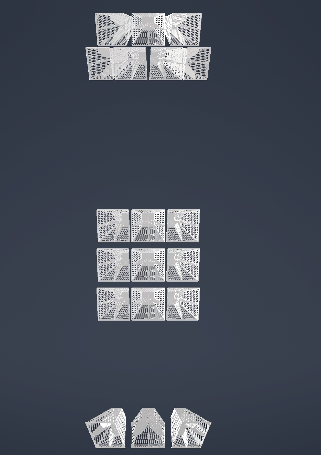
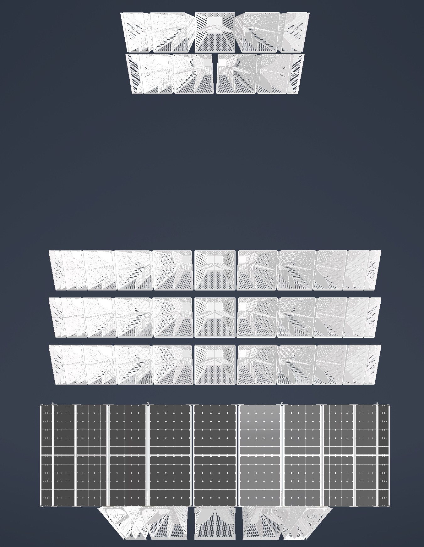
Amy | ANITA/PUEO pictures | Here are some ANITA/PUEO pictures that I received from Christian Mike that might be helpful. I include his descriptions as well.
The one with the black crates in the background is the ANITA 1 and ANITA 2 form factor and the one in the anechoic chamber is the ANITA 3 and ANITA 4 form factor. I dimensioned out an ANITA 3/4 antenna, in CAD space, to give you a better idea of the ridge profile. The ANITA 1/2 CAD models we have, I found, are inaccurate.
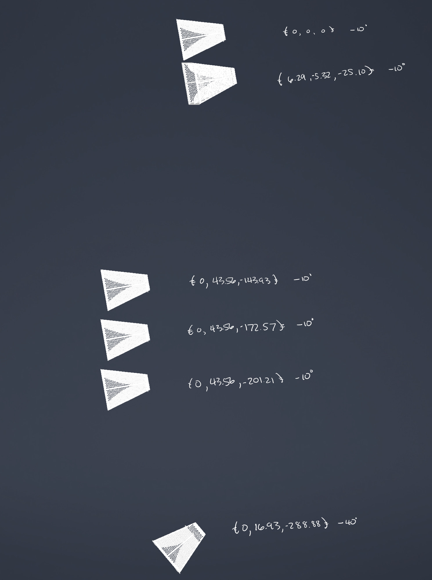
Attached are images of the PUEO antenna array geometry. One image annotates the approximate locations of the Vpol feed with the top antenna feed as the origin.
|
| Attachment 1: IMG_2362.jpg
|  |
| Attachment 2: IMG_2364.jpg
|  |
| Attachment 3: IMG_2365.jpg
|  |
|
|
201
|
Tue Mar 7 00:06:57 2023 |
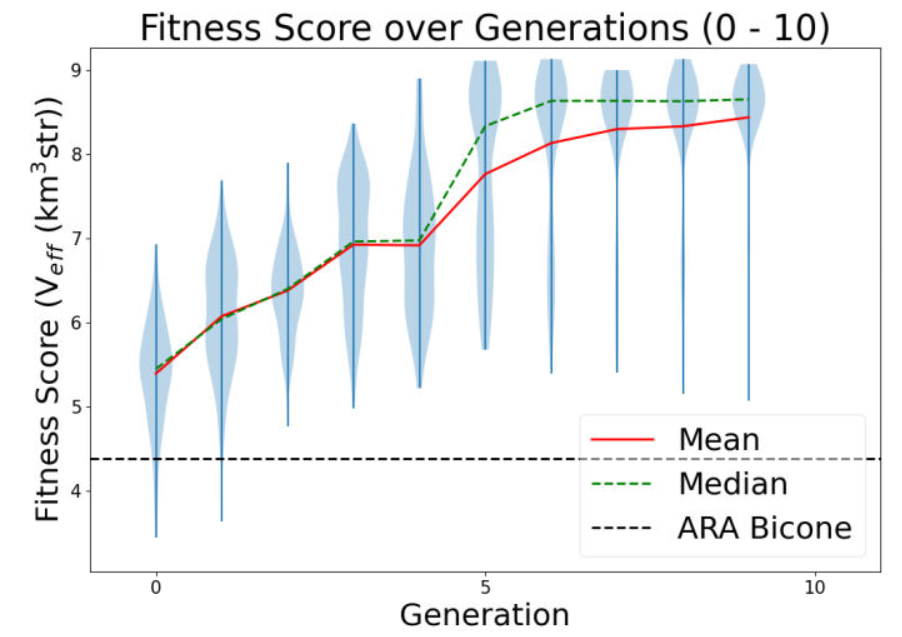
Bryan Reynolds | Retroactive AREA update: January 18, 2022 AREA run- No linear freq. dependence test w/ increased NPop | The following is a run summary of an AREA test using 100 individuals per generation, without the linear frequency dependence on the gain, with the frequency fixed (i.e. the same gain pattern is produced for all frequencies). This run was a preliminary test of the AREA algorithm with a larger NPop (100 individuals per generation) after seeing promising results in the previous test that only used 20 individuals per generation. The percentages of selection methods/operators used attempted to mimic the optimal percentages used for the PAEA Bicone Loop, but because the algorithms do not set these in the same manner, these are highly unlikely to be the best percentages to use. The results show a very quick plateau in fitness score with a loss in diversity of solutions after a low number of generations, potentially meaning that a poor breakdown of selection methods/operators was chosen. This result seems to underscore the need for a test loop-style optimization for AREA to determine the best breakdown of selection methods and operators to use for AREA.
Run details:
- Run Type
- Run Date
- Run Name
- 20230118breynoldsrun_noLinearDependAREATest_38RCO_2RM_58TCO_2TM_150000NNU_2Seeds
- Why are we doing this run?
- This test increased the number of individuals to 100 and attempted to mimic the percentages of selection methods and operators found to be optimal for the PAEA loop.
- What is different about this run from the last?
- The previous test showed slow/minimal evolution after ~12 generations, and it was speculated that this was due to a small NPop of 20 individuals. This test uses an increased NPop of 100 individuals.
- Symmetric, asymmetric, linear, nonlinear (what order):
- Number of individuals (NPOP):
- Number of neutrinos thrown in AraSim (NNT):
- 300,000 Total (150,000 NNU x 2 Seeds)
- Operatiors used (% of each):
- 96% Cross-Over, 4% Mutation
- Selection methods used (% of each):
- 40% Roullette, 60% Tournament
- Are we using the database?
Results:
- Summary and comments on results
- The fitness score quickly plaeaued and diversity of solutions was lost, potentially due to a unsuccessful choice of selection method and opterator percentages.
- An important future step is to work with Ryan to create a test loop optimization for the AREA algorithm, as it is written differently in how it is passed selection method and operator percentages and requires its own optimization to find the optimal ratios of these. (Work on creating a test loop optimization for AREA is currently underway).
EDIT 4/10/23
Re-uploading gain pattern associated with most fit individual from this run
|
| Attachment 1: 20230201_singleFreqTest_100NPop_fitnessPlot_10Gens.PNG
|  |
| Attachment 2: 20230410_AREA_mostFitIndivReUpload_singleFreqTest.PNG
|  |
|
|
200
|
Mon Mar 6 23:25:12 2023 |
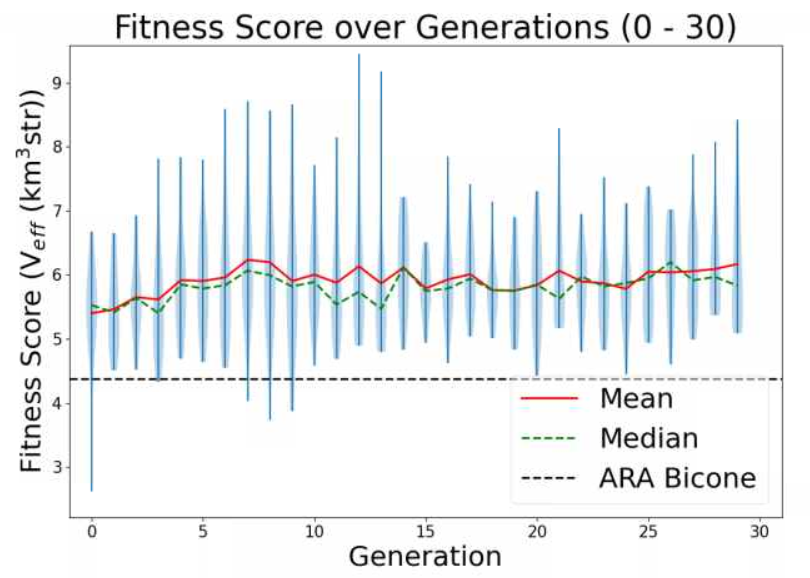
Bryan Reynolds | Retroactive AREA update: December 26, 2022 AREA run- No linear freq. dependence test | The following is a run summary of the AREA test without the linear frequency dependence on the gain, with the frequency fixed (i.e. the same gain pattern is produced for all frequencies). This run was a preliminary test of the AREA algorithm after fixing long-standing errors in the algorithm and finding that the initial constaints implemented did not work with the frequency dependence on gain. Results from this run did show a "proof-of-concept" that the AREA algorithm seems to evolve single frequencies in a promising way, however a low number of individuals may have stalled the evolution.
Run details:
- Run Type
- Run Date
- Run Name
- 20221226breynoldsrun_noLinearDependAREATest_8RCO_8RM_2TCO_2TM_30000NNU_10Seeds
- Why are we doing this run?
- We tested the AREA algorithm set to evolve at a single frequency in order to see if it would evolve a gain pattern at that frequency within the required constraints.
- What is different about this run from the last?
- This run only evolves gain patterns at a single frequency, allowing us to investigate the evolved gain patterns and check that the required constraints on the power conservation are met, without yet fixing the constraints function to work with the linear frequency dependence relationship. This is also the longest test run since the AREA algorithm was fixed and gotten into working order.
- Symmetric, asymmetric, linear, nonlinear (what order):
- Number of individuals (NPOP):
- Number of neutrinos thrown in AraSim (NNT):
- 300,000 Total (30,000 NNU x 10 Seeds)
- Operatiors used (% of each):
- 50% Cross-Over, 50% Mutation
- Selection methods used (% of each):
- 80% Roullette, 20% Tournament
- Are we using the database?
Results:
- Summary and comments on results
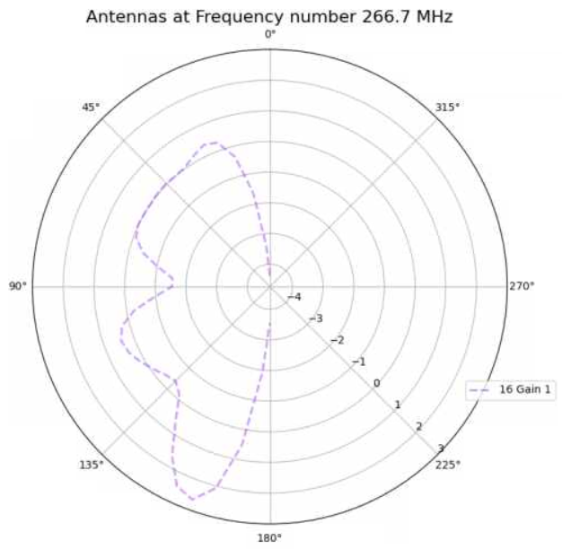
- The evolution appeared to be successful in that the most fit gain pattern found (attached) seems to make sense with our understanding of the underlying physics. Additionally, after inspecting the outputs, conservation of power was confirmed to be properly constrained. However, in the attached violin plot, the fitness score plateaued quickly and never evolved further, with the best individual coming in generation 12. This was speculated to be due to the small population used in this test (only 20 total individuals per generation).
|
| Attachment 1: 20230109_singleFreqTest_fitnessPlot_update30Gens.PNG
|  |
| Attachment 2: 20221229_singleFreqTest_overallBestIndiv_gen12Indiv17.PNG
|  |
|
|
Draft
|
Mon Mar 6 00:07:32 2023 |
Dylan Wells | Current Status of PUEO and To Do List for Hackathon | I went through the current PUEO Loop and documented everything that still needs to be accomplished before we can run.
Everything is compiled in this Google Doc which I will paste the current version of below.
Current Loop Overview:
Part A:
Runs GA, need to implement most recent GA (easy)
Part B:
B1:
Enters PUEO freq into simulation_PEC.xmacro then cats in PUEO simulationPECmacroskeletons.
Will need to update simulationPECmacroskeletons with XF script to simulate the Hpol and Vpol sides of the antenna separately.
The bash portion should be working.
B2:
Currently almost the same as the ARA version. Creates the output.xmacro and moves the uan files. Will most likely need to change to get files in PUEO/icemc format, ready for input into the conversion script.
Part C:
Runs conversion script XFintoPUEO.py
The Bash portion is complete. We will need simple modifications to XFintoPUEO.py depending on XF outputs.
Part D:
D1:
Changes setup file, runs IceMCCall_Array.sh batch job
Need make this batch job to change IceMC / PUEO to read in the correct files
(vv_0_{gen}_{i}, hh_0_{gen}_{i}) for the antenna i in generation gen.
I’ve commented where this should go. The rest of the job should be complete
The debug mode for D1 might not work, but it shouldn’t be necessary to run.
So, the bash portion should be able to run.
D2:
Currently confirms runs by looking at the number of files in the AraSimConfirmed directory and looks for specific AraSim errors.
This line will need to be changed to count the output files for icemc/pueo.
Change the error detection to just resubmit the job or something similar as we aren’t yet familiar with icemc errors during runtime.
Part E:
Runs the PUEO fitness function. Unfortunately, icemc doesn’t output error bars, so we will have to remake any plots reliant on that. Veffective is also the same as fitness score.
Currently it should be working with the basic needed plots for gain patterns and veffective scores. But, we should add some more cool, automatic plots.
Part F:
The plotting software seems to be specific to ARA output, needs PUEO versions.
ASYM LOOP:
Should be working with PUEO as a switch
IMPORTANT ISSUES:
Find out how to simulate polarization in XF:
Modify the current XF model, can be found in PAS1960/dylanwells1629/testproject.xf
The current model has all 4 sides of the antenna connected. However, the actual antenna is basically 2 antennas, one hpol and one vpol, electrically disconnected from each other. So, adjacent parts shouldn’t be electrically connected like they currently are in the model. We might have to simulate the two models independently. The goal for this portion is to figure out how to split up the antenna in the xmacro, and how to either simulate hpol and vpol separately or how to get xf to output hpol and vpol gain patterns.
XF Cross - Polarization, constraints --Alex
Make IceMC / PUEO read in out input gain patterns
Will need to modify Batch_Jobs/IceMCCallArray.sh to change icemc to read in the current gain files before running. You can find the conversion script in Antenna_Performance_Metric/XFintoPUEO.py and the batch job will be run in Loop_Parts/Part_D
We need to change icemc / pueo to read in the correct gain files before running it.
This will involve changing the anitaBuildTool/components/icemc/anita.cc ReadGains function starting on line 1413 to read in vv_0_{gen}_{num}, hh_0_{gen}_{num} , etc. (Do this with PueoSim) -- Dylan
I’m not sure if you will need to recompile these functions before running the icemc executable again, so find that out too. (enter pueoBuolder/ just run make) --Dylan
Make PUEO plotting software
All of the current plotting software is found within Part_E and Part_F. Sadly, icemc does not output errors for the veffectives (at least not that I could find, maybe you can find it), so much of the Ara plotting software will not work with PUEO outputs. The fitness scores csv will be the same format as ARA’s, and veffectives will be the same as fitness scores for PUEO. Figure out how to change the existing ARA python plotting scripts or make new ones. --Bryan
Find out how to run PEUOsim and document outputs
Currently the loop is working with icemc, but we want to use PUEOsim for the future. So, document installing it, running it, and the outputs. (inputs are the same as icemc) -- Dylan |
|
|
198
|
Fri Feb 24 10:05:38 2023 |
Alex M | Paper Symmetric Run for Reviewer | We began a new run for a symmetric bicone antenna. The purpose of this is to satisfy the most recent comments from the reviewer on the paper. We are using the same GA as for the paper with the same parameters. I will update this post soon with more details about this run. There is a run_details file attached, but please wait for me to update this post with more specifics as the version of the GA being used is less connected to the details presented in that file.
The data can be found here: /fs/ess/PAS1960/BiconeEvolutionOSC/BiconeEvolution/current_antenna_evo_build/XF_Loop/Evolutionary_Loop/Run_Outputs/2023_02_20_Symmetric_Run . |
| Attachment 1: run_details_2023_02_20_Symmetric_Run.txt
|
####### VARIABLES: LINES TO CHECK OVER WHEN STARTING A NEW RUN ###############################################################################################
RunName='2023_02_20_Symmetric_Run'      ## This is the name of the run. You need to make a unique name each time you run.
TotalGens=100                   ## number of generations (after initial) to run through
NPOP=50                         ## number of individuals per generation; please keep this value below 99
Seeds=10                        ## This is how many AraSim jobs will run for each individual## the number frequencies being iterated over in XF (Currectly only affects the output.xmacro loop)
FREQ=60                         ## the number frequencies being iterated over in XF (Currectly only affects the output.xmacro loop)
NNT=30000                       ## Number of Neutrinos Thrown in AraSim
exp=18                          ## exponent of the energy for the neutrinos in AraSim
ScaleFactor=1.0                 ## ScaleFactor used when punishing fitness scores of antennae larger than the drilling holes
GeoFactor=1                     ## This is the number by which we are scaling DOWN our antennas. This is passed to many files
num_keys=4                      ## how many XF keys we are letting this run use
database_flag=0                 ## 0 if not using the database, 1 if using the database
                                ## These next 3 define the symmetry of the cones.
RADIUS=0                        ## If 1, radius is asymmetric. If 0, radius is symmetric
LENGTH=0                        ## If 1, length is asymmetric. If 0, length is symmetric
ANGLE=0                         ## If 1, angle is asymmetric. If 0, angle is symmetric
CURVED=0                        ## If 1, evolve curved sides. If 0, sides are straight
A=0                             ## If 1, A is asymmetric
B=0                             ## If 1, B is asymmetric
SEPARATION=0                    ## If 1, separation evolves. If 0, separation is constant
NSECTIONS=1                     ## The number of chromosomes
DEBUG_MODE=0                    ## 1 for testing (ex: send specific seeds), 0 for real runs
                                ## These next variables are the values passed to the GA
REPRODUCTION=3                  ## Number (not fraction!) of individuals formed through reproduction
CROSSOVER=36                    ## Number (not fraction!) of individuals formed through crossover
MUTATION=25                     ## Probability of mutation (divided by 100)
SIGMA=6                         ## Standard deviation for the mutation operation (divided by 100)
ROULETTE=8                      ## Percent of individuals selected through roulette (divided by 10)
TOURNAMENT=2                    ## Percent of individuals selected through tournament (divided by 10)
RANK=0                          ## Percent of individuals selected through rank (divided by 10)
ELITE=0                         ## Elite function on/off (1/0)

#####################################################################################################################################################
|
|
|
197
|
Mon Feb 20 12:33:20 2023 |
Dennis H. Calderon | AraSim Simulations for Top 5 Antennas (12/2022) with Higher Stats | AraSim Simulations for Top 5 Antennas from 12/2022 Run with 3 million simulated events
Simulated using Arasim version currently used in GENETIS Loop
/fs/ess/PAS1960/BiconeEvolutionOSC/AraSim/
AraSim ROOT files stored in
/fs/ess/PAS1960/ROOT_Files_Higher_Stats/AraSim_Loop_122022/Feb_2023_Crazy_Sides/
Antennas simulated
- Generation: 13, Individual: 84
- Generation: 18, Individual: 89
- Generation: 19, Individual: 96
- Generation: 29, Individual: 87
- Generation: 9, Individual: 50
Results
| Antenna |
Total Events |
Triggered Events |
Weighted Events |
Effective Volume |
Effective Volume Error |
| 13_84 |
2995982 |
40251 |
16058 |
5.71 |
0.035 |
| 18_89 |
3010000 |
40224 |
15963 |
5.65 |
0.035 |
| 19_96 |
3010000 |
39989 |
16034 |
5.68 |
0.031 |
| 29_87 |
3010000 |
40056 |
16049 |
5.68 |
0.034 |
| 9_50 |
3010000 |
40042 |
16057 |
5.69 |
0.034 |
| ARA_Sym_Bicone_6in |
3010000 |
36627 |
14334 |
5.08 |
0.032 |
Conclusion
Antenna from Generation 13 Individual 84 performed the best with these stats |
| Attachment 1: Crazy_Sides_Triggered_Event_Data.pdf
|
|
|
196
|
Sun Feb 19 17:12:34 2023 |
Jack Tillman | Physics Plots - 9_50, 13_84, 18_89, 19_96, 29_87 | Attached is a pdf of physics plots generated for the 9_50, 13_84, 18_89, 19_96, and 29_87 crazy sides individuals along with another containing information on the amount of triggered events and effective volumes for each individual. The crazy sides individuals were simulated for 3 million events using the same Arasim version as is currently in the loop. |
| Attachment 1: Feb2023_Physics_Plots_Powerpoint.pdf
|
| Attachment 2: Crazy_Sides_Triggered_Event_Data.pdf
|
|
|
195
|
Wed Feb 15 16:33:17 2023 |
Jacob Weiler | pueoSim Input Files | Input File Format for pueoSim (Also ICEMC)
Frequency Range: From 200 MHz to 1500 MHz incrementing by 10 MHz steps
There are 8 different files that are required for pueoSim. They are:
vv_0: Max Gain at each Frequency, Vertical Polarization
hh_0: Max Gain at each Frequency, Horizontal Polarization
vh_0: Max Gain at each Frequency, Vertical to Horizontal Polarization
hv_0: Max Gain at each Frequency, Horizontal to Vertical Polarization
vv_el: Gain at Theta Angles [5, 10, 20, 30, 45, 90] for each Frequency, Vertical Polarization
vv_az: Gain at Phi Angles [5, 10, 20, 30, 45, 90] for each Frequency, Vertical Polarization
hh_el: Gain at Theta Angles [5, 10, 20, 30, 45, 90] for each Frequency, Horizontal Polarization
hh_az: Gain at Phi Angles [5, 10, 20, 30, 45, 90] for each Frequency, Horizontal Polarization
Currently XF doesn't output all the information we need to create all these files. The only files able to be made from current XF outputs are vv_0, vv_el, and vv_az. Once we have the correct XF Outputs, it shouldn't be too much of a hassle to fix the current translation code.
Format for each of the files are the same. One column is Frequency (Hz) and the other is Gain. Attached are example files vv_0 and vv_el to visually see the format, though the frequency range is the current ARA range and not the final PUEO range as I am using ARA data to make these files. The files are named vv_0 (no .txt or .csv or any extension) and vv_el
Link to Google Doc with this information: https://docs.google.com/document/d/1iRUF6hIEyQfMK0LL21caRuHPgXYP30ZdkSkFv_-Y8R0/edit |
| Attachment 1: vv_0_1
|
8.33e+07 2.11822
1.00e+08 0.9436538
1.17e+08 1.205556
1.33e+08 2.149637
1.50e+08 2.729287
1.67e+08 2.619639
1.83e+08 2.532374
2.00e+08 2.289813
2.17e+08 2.406259
2.33e+08 2.442176
2.50e+08 2.628373
2.67e+08 2.359219
2.83e+08 1.761219
3.00e+08 1.502431
3.17e+08 2.106109
3.33e+08 2.71283
3.50e+08 3.247887
3.67e+08 3.524175
3.83e+08 3.615199
4.00e+08 3.448137
4.17e+08 3.003371
4.33e+08 2.217343
4.50e+08 0.9601937
4.67e+08 -0.757537
4.83e+08 -3.06678
5.00e+08 -5.635237
5.17e+08 -8.2271
5.33e+08 -9.618924
5.50e+08 -9.791239
5.67e+08 -9.201792
5.83e+08 -9.086395
6.00e+08 -9.560636
6.17e+08 -10.94548
6.33e+08 -13.11583
6.50e+08 -16.3255
6.67e+08 -22.45401
6.83e+08 -34.91041
7.00e+08 -18.52293
7.17e+08 -12.31584
7.33e+08 -8.076791
7.50e+08 -5.287256
7.67e+08 -3.399354
7.83e+08 -2.394224
8.00e+08 -2.031315
8.17e+08 -2.07204
8.33e+08 -2.531995
8.50e+08 -3.185455
8.67e+08 -4.223504
8.83e+08 -5.275337
9.00e+08 -6.274862
9.17e+08 -6.532893
9.33e+08 -6.242696
9.50e+08 -5.514515
9.67e+08 -4.831669
9.83e+08 -4.240883
1.00e+09 -3.779134
1.02e+09 -3.558248
1.03e+09 -3.38254
1.05e+09 -3.543484
1.07e+09 -3.611961
|
| Attachment 2: vv_el_1
|
8.33e+07 -19.61153
1.00e+08 -21.05896
1.17e+08 -21.14054
1.33e+08 -20.63561
1.50e+08 -20.56293
1.67e+08 -21.11712
1.83e+08 -21.6924
2.00e+08 -22.23107
2.17e+08 -22.38623
2.33e+08 -22.01034
2.50e+08 -20.95566
2.67e+08 -19.49215
2.83e+08 -19.23056
3.00e+08 -21.02166
3.17e+08 -24.84512
3.33e+08 -30.42641
3.50e+08 -30.39998
3.67e+08 -24.79053
3.83e+08 -20.92692
4.00e+08 -18.28975
4.17e+08 -16.42205
4.33e+08 -15.10437
4.50e+08 -14.27861
4.67e+08 -13.84517
4.83e+08 -13.72481
5.00e+08 -13.71555
5.17e+08 -13.67698
5.33e+08 -13.47088
5.50e+08 -13.12691
5.67e+08 -12.80078
5.83e+08 -12.76288
6.00e+08 -13.29937
6.17e+08 -14.53883
6.33e+08 -16.51551
6.50e+08 -19.31712
6.67e+08 -23.38054
6.83e+08 -28.77149
7.00e+08 -26.26056
7.17e+08 -20.68733
7.33e+08 -16.92428
7.50e+08 -14.40974
7.67e+08 -12.83548
7.83e+08 -11.95044
8.00e+08 -11.46287
8.17e+08 -11.11874
8.33e+08 -10.75576
8.50e+08 -10.35075
8.67e+08 -9.963577
8.83e+08 -9.712427
9.00e+08 -9.691508
9.17e+08 -9.958833
9.33e+08 -10.48243
9.50e+08 -11.25391
9.67e+08 -12.16331
9.83e+08 -13.22009
1.00e+09 -14.23114
1.02e+09 -15.10789
1.03e+09 -15.45052
1.05e+09 -15.20106
1.07e+09 -14.44125
8.33e+07 -13.61057
1.00e+08 -15.05177
1.17e+08 -15.12521
1.33e+08 -14.60951
1.50e+08 -14.52322
1.67e+08 -15.06334
1.83e+08 -15.62302
2.00e+08 -16.1491
2.17e+08 -16.29245
2.33e+08 -15.91477
2.50e+08 -14.8618
2.67e+08 -13.39692
2.83e+08 -13.1095
3.00e+08 -14.84329
3.17e+08 -18.54948
3.33e+08 -24.02788
3.50e+08 -24.85216
3.67e+08 -19.17134
3.83e+08 -15.1775
4.00e+08 -12.46181
4.17e+08 -10.53846
4.33e+08 -9.176889
4.50e+08 -8.313917
4.67e+08 -7.849362
4.83e+08 -7.705056
5.00e+08 -7.681289
5.17e+08 -7.638247
5.33e+08 -7.434054
5.50e+08 -7.090922
5.67e+08 -6.756147
5.83e+08 -6.694556
6.00e+08 -7.188318
6.17e+08 -8.361327
6.33e+08 -10.23697
6.50e+08 -12.87492
6.67e+08 -16.64803
6.83e+08 -21.92072
7.00e+08 -21.02616
7.17e+08 -15.29548
7.33e+08 -11.32251
7.50e+08 -8.680712
7.67e+08 -7.026238
7.83e+08 -6.092156
8.00e+08 -5.577537
8.17e+08 -5.222755
8.33e+08 -4.855792
8.50e+08 -4.445815
8.67e+08 -4.04485
8.83e+08 -3.769133
9.00e+08 -3.712655
9.17e+08 -3.934655
9.33e+08 -4.405427
9.50e+08 -5.116381
9.67e+08 -5.962245
9.83e+08 -6.955142
1.00e+09 -7.921253
1.02e+09 -8.79726
1.03e+09 -9.21963
1.05e+09 -9.101768
1.07e+09 -8.46457
8.33e+07 -7.672357
1.00e+08 -9.089356
1.17e+08 -9.131313
1.33e+08 -8.574198
1.50e+08 -8.436004
1.67e+08 -8.923278
1.83e+08 -9.424584
2.00e+08 -9.903976
2.17e+08 -10.00275
2.33e+08 -9.618365
2.50e+08 -8.573076
2.67e+08 -7.108304
2.83e+08 -6.730207
3.00e+08 -8.258189
3.17e+08 -11.54483
3.33e+08 -16.48101
3.50e+08 -20.44362
3.67e+08 -14.99668
3.83e+08 -10.39325
4.00e+08 -7.322492
4.17e+08 -5.15867
4.33e+08 -3.614434
4.50e+08 -2.600771
4.67e+08 -2.012469
4.83e+08 -1.773685
5.00e+08 -1.692136
5.17e+08 -1.631185
5.33e+08 -1.436829
5.50e+08 -1.104481
5.67e+08 -0.7477778
5.83e+08 -0.6082266
6.00e+08 -0.9526983
6.17e+08 -1.891183
6.33e+08 -3.416407
6.50e+08 -5.508213
6.67e+08 -8.350483
6.83e+08 -12.36274
7.00e+08 -15.94441
7.17e+08 -11.94184
7.33e+08 -7.215725
7.50e+08 -4.031596
7.67e+08 -2.033106
7.83e+08 -0.8896422
8.00e+08 -0.2599349
8.17e+08 0.1364451
8.33e+08 0.508579
8.50e+08 0.9189453
8.67e+08 1.351561
8.83e+08 1.703014
9.00e+08 1.881713
9.17e+08 1.823472
9.33e+08 1.546895
9.50e+08 1.061567
9.67e+08 0.4561304
9.83e+08 -0.2820854
1.00e+09 -1.030102
1.02e+09 -1.782719
1.03e+09 -2.307445
1.05e+09 -2.516682
1.07e+09 -2.306051
8.33e+07 -4.297208
1.00e+08 -5.677257
1.17e+08 -5.671377
1.33e+08 -5.051709
1.50e+08 -4.836023
1.67e+08 -5.245572
1.83e+08 -5.661229
2.00e+08 -6.072461
2.17e+08 -6.104968
2.33e+08 -5.710936
2.50e+08 -4.682109
2.67e+08 -3.235083
2.83e+08 -2.745363
3.00e+08 -3.999428
3.17e+08 -6.728222
3.33e+08 -10.71871
3.50e+08 -16.85379
3.67e+08 -15.67102
3.83e+08 -9.610837
4.00e+08 -5.713407
4.17e+08 -3.051436
4.33e+08 -1.161082
4.50e+08 0.1202912
4.67e+08 0.9189369
4.83e+08 1.315152
5.00e+08 1.493735
5.17e+08 1.58528
5.33e+08 1.756137
5.50e+08 2.045786
5.67e+08 2.395989
5.83e+08 2.609925
6.00e+08 2.448707
6.17e+08 1.814713
6.33e+08 0.7368893
6.50e+08 -0.702895
6.67e+08 -2.543868
6.83e+08 -4.926394
7.00e+08 -7.929486
7.17e+08 -9.722289
7.33e+08 -6.876765
7.50e+08 -3.230588
7.67e+08 -0.6956752
7.83e+08 0.8078526
8.00e+08 1.641694
8.17e+08 2.100993
8.33e+08 2.439688
8.50e+08 2.768471
8.67e+08 3.145787
8.83e+08 3.516955
9.00e+08 3.809434
9.17e+08 3.95456
9.33e+08 3.942741
9.50e+08 3.779913
9.67e+08 3.52297
9.83e+08 3.16981
1.00e+09 2.79626
1.02e+09 2.387999
1.03e+09 2.060452
1.05e+09 1.836171
1.07e+09 1.800864
8.33e+07 -1.144795
1.00e+08 -2.455938
1.17e+08 -2.361629
1.33e+08 -1.627502
1.50e+08 -1.273074
1.67e+08 -1.547562
1.83e+08 -1.814825
2.00e+08 -2.110694
2.17e+08 -2.028768
2.33e+08 -1.626653
2.50e+08 -0.6542816
2.67e+08 0.689521
2.83e+08 1.297091
3.00e+08 0.4526482
3.17e+08 -1.408842
3.33e+08 -3.855139
3.50e+08 -7.45269
3.67e+08 -13.8242
3.83e+08 -21.86369
4.00e+08 -10.18875
4.17e+08 -4.926253
4.33e+08 -1.717269
4.50e+08 0.408406
4.67e+08 1.793992
4.83e+08 2.602153
5.00e+08 3.033494
5.17e+08 3.210672
5.33e+08 3.304456
5.50e+08 3.387133
5.67e+08 3.514676
5.83e+08 3.634609
6.00e+08 3.636984
6.17e+08 3.453297
6.33e+08 3.09098
6.50e+08 2.620621
6.67e+08 2.051623
6.83e+08 1.398647
7.00e+08 0.6288801
7.17e+08 -0.2089145
7.33e+08 -0.8729058
7.50e+08 -0.8983268
7.67e+08 -0.1494044
7.83e+08 0.8073187
8.00e+08 1.548733
8.17e+08 1.943862
8.33e+08 2.050232
8.50e+08 1.890077
8.67e+08 1.512847
8.83e+08 0.9992631
9.00e+08 0.4794029
9.17e+08 0.180576
9.33e+08 0.1580454
9.50e+08 0.4193046
9.67e+08 0.7895336
9.83e+08 1.223261
1.00e+09 1.625476
1.02e+09 2.006417
1.03e+09 2.338812
1.05e+09 2.613677
1.07e+09 2.839776
... 61 more lines ...
|
|
|
194
|
Mon Feb 13 14:56:57 2023 |
Jack Tillman | Building - Physics Plots for 9_50, 13_84, 18_89, 19_96, 29_87 Antennae | Physics plots were created for 300K events from the higher statistic simulation results for the 9_50, 13_84, 18_89, 19_96, and 29_87 antennae.
The simulation was inaccurate because a discrepancy exists between the higher simulation physics plots and the physics plots created for the 300K event results currently in the GENETIS Loop. This can be seen in the attached pdf file.
The simulation may have been inaccurate due to incorrect gain files.
The higher statistic simulations must be rerun for the 9_50, 13_84, 18_89, 19_96, and 29_87 antennae.
|
| Attachment 1: Genetis_Physics_Plot_Comparison_Slides.pdf
|
|
|
193
|
Fri Feb 10 15:55:53 2023 |
Jack Tillman | Building - Matching Circuit PCB | I've completed laying out the PCB for the 14-rung matching circuit. Attached are png files of two PCB designs. One uses LPS5050 inductors while the other uses LPS6235 inductors. The dimensions shown are in millimeters. |
| Attachment 1: LPS5050_Dimensioned_PCB.png
|  |
| Attachment 2: LPS6235_Dimensioned_PCB.png
|  |
|