| |
ID |
Date |
Author |
Subject |
|
|
243
|
Mon Jun 2 14:10:59 2025 |
Jacob Weiler | Building Status 06/02/2025 | We are almost to where we can start the physical building of the antenna!
I've attached all the information I currently have regarding the building project. Some of it is messy work notes and some is well-structured.
I’ve attached the following files for the GENETIS building project:
- Building Dump.txt
- My working notes that I used while trying to simulate the antenna in XFdtd (very messy)
- Building Dump of Useful Materials.txt
- List of materials that I found regarding the building project like slides, elogs, etc.
- Simulating Building Model.txt
- A writeup I made describing my process for simulating the antenna in XFdtd
- Done with change materials.zip
- Solidworks model of antenna
I also made a slide deck that contains the directory locations + has graphs HERE. |
| Attachment 1: Building_Dump_of_Useful_Materials.txt
|
Building Dump:

For Initial Building Run:
Generation 13, individual 84 seems to be result being used (this assumption is based on the fact that when trying to straighten the sides for building they used this individual)
	/fs/ess/PAS1960/BiconeEvolutionOSC/BiconeEvolution/current_antenna_evo_build/XF_Loop/Evolutionary_Loop/Run_Outputs/2022_12_29

Elog Links for first building runs:
	- Run Details: https://radiorm.physics.ohio-state.edu/elog/GENETIS/188
	- Run Results + Gain Patterns: https://radiorm.physics.ohio-state.edu/elog/GENETIS/189
	- Matching Circuit PCB: https://radiorm.physics.ohio-state.edu/elog/GENETIS/193
	- Matching Circuit Parts: https://radiorm.physics.ohio-state.edu/elog/GENETIS/191
	- Matching Circuit Schematic: https://radiorm.physics.ohio-state.edu/elog/GENETIS/230
	- Matching Circuit Initial Design: https://radiorm.physics.ohio-state.edu/elog/GENETIS/183
	- PoR Plots 1: https://radiorm.physics.ohio-state.edu/elog/GENETIS/194
	- PoR Plots 2: https://radiorm.physics.ohio-state.edu/elog/GENETIS/196
	- Straightened Sides 1: https://radiorm.physics.ohio-state.edu/elog/GENETIS/229
	- Straightened Sides 2: https://radiorm.physics.ohio-state.edu/elog/GENETIS/236
	- Engineering Call: https://docs.google.com/presentation/d/1Lo_6mFTmPbkToTrEeOpvznSdbxyPZexPag1qijTeYyM/edit?usp=sharing


At some point for some reason, another run seems to have been created for building with the crazy sides run here:
/fs/ess/PAS1960/BiconeEvolutionOSC/BiconeEvolution/current_antenna_evo_build/XF_Loop/Evolutionary_Loop/Run_Outputs/2023_09_05_realized_curved_run

Top 5 vEffective Scores:
Value: 5.09897, Generation: 41, Individual: 44 (Seems to be this one, modified)
Value: 5.07746, Generation: 37, Individual: 16
Value: 5.05508, Generation: 37, Individual: 5
Value: 5.04558, Generation: 38, Individual: 12
Value: 5.04026, Generation: 48, Individual: 5


GENETIS Useful Links:
	- GENETIS Google Drive: https://drive.google.com/drive/folders/1iDamk46R2_oOLHtvsOg4jNy05mCiB7Sn?dmr=1&ec=wgc-drive-hero-goto
	- Onboarding Materials: https://radiorm.physics.ohio-state.edu/elog/GENETIS/41
	- Julie's Dissertation: https://radiorm.physics.ohio-state.edu/elog/Write-Ups/220404_161525/Julie_Rolla_Dissertation.pdf
	- Julie's Candidacy: https://as-phy-radiorm.asc.ohio-state.edu/elog/Write-Ups/44
	- ICRC Proceedings: https://arxiv.org/pdf/2112.00197
	- Phys Rev D Paper: https://journals.aps.org/prd/abstract/10.1103/PhysRevD.108.102002
	- ARA Loop GitHub: https://github.com/osu-particle-astrophysics/GENETIS-ARA
	- PUEO Loop GitHub: https://github.com/osu-particle-astrophysics/GENETIS_PUEO
	- Shared Code GitHub: https://github.com/osu-particle-astrophysics/Shared-Code
	- AraSim GitHub: https://github.com/ara-software/AraSim/tree/master
	- pueoSim GitHub: https://github.com/PUEOCollaboration/pueoSim
|
| Attachment 2: Simulating_Building_Model.txt
|
Simulating Building Model

Getting the model we want to build from Solidworks into XF ready for simulations took a bit of work. Here are the steps and things I did to get it to finally work with materials and everything enabled (minus conductors in the coax cable).

General Instructions to setup the antenna the same as I did. Saving after each of these steps.

Getting out of Solidworks:
To get out of Solidworks, I used .step file under the assumption that it would carry the material data over into XF (this assumption was based on what I had read online, though I was looking at the wrong places for that information as I found out later). With this assumption, we spent time getting the materials correct in Solidworks before exporting out into the .step file. I spent considerable time double checking the materials in Solidworks to make sure that everything was defined correctly with at least good enough approximations of the materials to get a simulation working.

Material definitions:

    Shells: Plastic wrapped in Copper Foil, approximated by just having the whole shell as Copper

    Screws Connecting horizontal halves: ABS (PEEK Plastic)

    Supports Connecting vertical halves: ABS

    Other screws: Non-magnetic stainless steel (Passivated 18-8 Stainless Steel)

    Coax Cable:

        Dielectric: Foam Polyethylene (FPE)

        Inner Conductor: Solid Bare Copper Covered Aluminum

        Outer Conductor: Aluminum Tape

        Outer Braid: Tinned Copper

        Jacket: Polyethylene

    Everything else: Approximated as copper (not entirely sure if they are copper fully or if they are just wrapped with copper foil)

Importing into XFdtd:
After having the step file exported, I put the file onto OSC and opened a new XFdtd project. I then clicked the "Import -> Cad Models" to select my file and have it imported. I did not import in the material data as I found out it did not import in correctly to each part, so I ignored it and manually added the material definitions later.

I now have the model into XFdtd, but it’s rotated 90 degrees to be in the horizontal plane. This isn’t inherently bad, but I want my surrounding scripts to not have to be changed much so I rotate the model to have the wire pointing in the +z direction in XFdtd. Once I’ve done this, I right click on the Braid and Inner + Outer conductors in the coax cable and select something similar to "Do not include in meshing." This now makes sure that these are NOT in the simulation.

Then, I manually added material properties into XFdtd from definitions I looked up online for the electric + magnetic properties of:

    Copper

    Plastic (ABS)

    Foam Polyethylene (dielectric)

    Polyethylene

    Aluminum

    Stainless Steel

After creating these material definitions, I applied them to the appropriate parts.

Feed adjustments:
I want the feed to be in the same location as the coax cable for the best results, problem is that there are holes in the place where the coax cable would be split (which I disabled to prevent shorting!). So, I setup two copper pucks (not much thicker than the copper pieces that cover the tops by the feeds) to fill out the holes and make sure each half is connected to each corresponding side of the feed. After I place these in the correct location, I use the same 50-ohm feed setup script used in the GENETIS Vpol loop.

Now we have everything almost ready to simulate.

Simulation Setup:
There are various things needed to be done to setup the script, and while you can use the GUI, I’m not familiar enough with it so I just used the corresponding scripts in the GENETIS loop that would be needed before an XF simulation takes place. After I run this, we are now ready to simulate.

Running Simulation:
Again, not familiar with the GUI so I just used the GENETIS XFdtd job scripts and modified them for this purpose (which was just adjusting directories of outputs). Then I submitted the job and waited for it to complete (I believe it took around 8 min per simulation for this antenna).

Getting uan files:
I then opened the simulation and ran the same code used to output UANs as used in the GENETIS loop to output all 60 uan files at the frequencies we want.

Now you should have the files for the building model that was made in CAD!

Debugging Steps I took:
This took me a while over spring break, at least a lot longer than I thought it would.

    I found out that the material data from .step file does not translate as I had expected into XFdtd so I had to manually input the material data as shown above

    I found out that hiding a part in XF does NOT exclude it from simulation, you have to remove it from meshing or it still remains there

    I did compare the geometries between the as-evolved antenna and this building model, there are differences but they are slight. Overall they are very similar

    Removing the conductors for the coax cable is necessary as it will just short the two pieces (leading back to 2) which makes sense

Final:
After doing all this, I ended up getting what I deemed reasonable for the outputs for the building model after 28 runs in my 03_13_2025_manual.xf xf file on my user. Run28 is the run that I describe setting up above this text.

The material is not 1-1 with what will be built as I found it difficult to find exact electro-magnetic properties for all of these, so maybe the discrepancies in gain could be resolved through more rigorous definitions. It could actually technically make it worse, but maybe when this is physically built this will need to be done to get more accurate results to compare against.

Simulating both of these with higher statistics in AraSim resulted in the antennas actually performing worse than the base Vpol antenna, which stinks but it is both of the antennas not just one!

After (delayed) emails back and forth with Christian Miki from University of Hawaii, he found these same issues while he was looking at the model from CAD before I went through the XFdtd simulation steps.

Material Definitions in XF:
For critique, here are the material definitions I used in the XF simulation (using XF material definition windows). You should be able to look at them in the actual xf project I mentioned above in my user (full path in slide decks)

All setup with the following:
Type: Physical
Electric: Isotropic
Magnetic: Isotropic

Passivated 18-8 Stainless Steel:
Electric Tab
Type: Nondispersive
Entry Method: Normal
Good Conductor: Automatic
Conductivity: 1.1e+06 S/m
Relative Permittivity: 1
Infinite Dielectric Strength: Yes

Magnetic Tab
Type: Nondispersive
Entry Method: Normal
Conductivity: 0
Relative Permeability: 1.03

PEEK Plastic
Electric Tab
Type: Nondispersive
Entry Method: Loss Tangent
Good Conductor: Automatic
Relative Permittivity: 3.3
Loss Tangent: 0.003
Evaluation Frequency: 1 MHz
Infinite Dielectric Strength: Yes

Magnetic Tab
Type: Nondispersive
Entry Method: Normal
Conductivity: 0
Relative Permeability: 1

Foam Polyethylene
Electric Tab
Type: Nondispersive
Entry Method: Loss Tangent
Good Conductor: Automatic
Relative Permittivity: 1.6
Loss Tangent: 0.0004
Evaluation Frequency: 1 MHz
Infinite Dielectric Strength: Yes

Magnetic Tab
Type: Nondispersive
Entry Method: Normal
Conductivity: 0
Relative Permeability: 1

Polyethylene
Electric Tab
Type: Nondispersive
Entry Method: Loss Tangent
Good Conductor: Automatic
Relative Permittivity: 2.25
Loss Tangent: 0.0004
Evaluation Frequency: 1 MHz
Infinite Dielectric Strength: Yes

Magnetic Tab
Type: Nondispersive
Entry Method: Normal
Conductivity: 0
Relative Permeability: 1

ABS Plastic
Electric Tab
Type: Nondispersive
Entry Method: Loss Tangent
Good Conductor: Automatic
Relative Permittivity: 3.2
Loss Tangent: 0.005
Evaluation Frequency: 1 MHz
Infinite Dielectric Strength: Yes

Magnetic Tab
Type: Nondispersive
Entry Method: Normal
Conductivity: 0
Relative Permeability: 1

Copper Foil
Electric Tab
Type: Nondispersive
Entry Method: Normal
Good Conductor: Automatic
Conductivity: 5.96e+07 S/m
Relative Permittivity: 1
Infinite Dielectric Strength: Yes

Magnetic Tab
Type: Nondispersive
Entry Method: Normal
Conductivity: 0
Relative Permeability: 1
|
| Attachment 3: Building_Dump.txt
|
Building Dump:
Debugging Issues with Antenna model simulation:

Graphs to get (compared to Curved_Sides Antenna Run):
- Gain Plots
	- Look at frequencies where dips. Could be due to: dielectric loss, mismatched impedance or structural changes
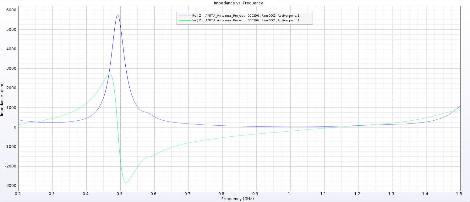
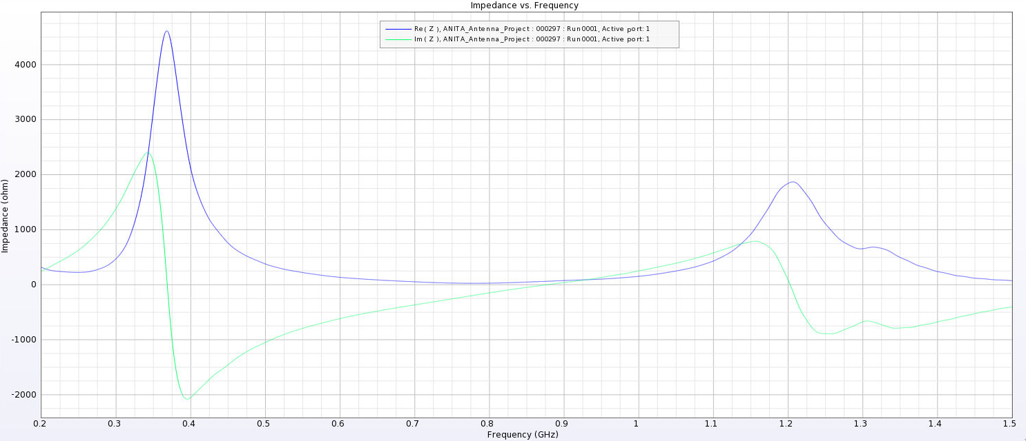
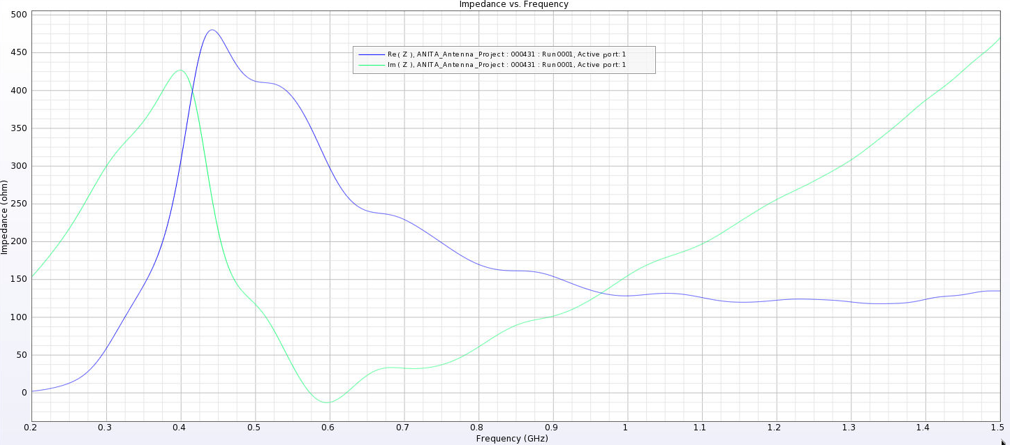
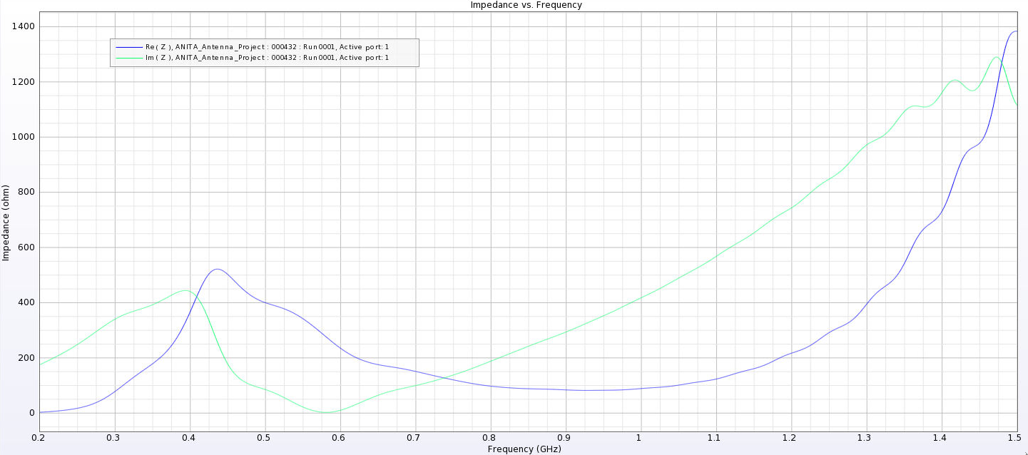
- Impedance Over Frequency Plots
	- Want impedance to be around 50 Ohm for resistive components and 0 for reactance at operational frequencies
- S11 Plots (Return Loss VS Frequency)
	- Look for where the S11 dips to determine where the antenna is resonant
- Total Efficiency Vs Frequencies
	- Drops at certain frequencies indicates problems!
- VSWR vs Frequency
	- Lower VSWR means better matching


in 03_13_2025_manual.xf:
Run1 = wrong material defs (deleted)
Run2 = glitched it
Run3 = wrong material def again slightly changed tho
Run4 = wrong material, with conductor gone
Run5 = wrong material, with full wire gone
Run6 = right material, full wire gone
Run7 = right material, conductor gone
Run8 = right material, everything there feed shifted to side
Run9 = right material, feed in middle of conductor
Run10 = right material, wire gone feed offset reduced (putting closer to center). this failed because the top of the feed was disconnected
Run11 = right material, feed with correct max feed offset allowed, coax gone
Run12 = trying the same thing but with the coax gone with building the feed
Run13 = with coax cable back, feed shifted closer to middle (apparently forgot to save and it's just the same thing.. as run12)
Run14 = adding pads and putting feed in the middle of the antenna, leave dielectric and jacket turned on
Run16 = pads, feed in middle, removing dielectric and jacket (-300 thing again.. not sure why)
Run17 = same thing but ABS material changed and adjusted pucks a little
Run18 = same ABS material change but with only inner conductor removed (I am testing why I am getting -300..)
Run19 = removed supports, still  with pucks + only inner conductor removed
Run20 = removing pucks, with conductor removed and new ABS material (no more -300 but very low again...)
run21 = removed pucks, conductors(PLURAL) with new ABS Material
run23 = back to just supports, offset feed new ABS Material
run24 = coax gone, og ABS material, with the offset feed closer to the middle
run25 = everything back to normal coax gone (something wrong)
run26 = trying to fix the issue I'm seeing (FIXED) you have to uncheck that materials are included in meshing :/
run27 = actually removing the outer and inner conductors (yields worse gains!)
run28 = moving to feed center w/ copper plates and with the jacket + dielectric

Seems like the wire in the middle should be plastic (or non-conducting)? based off document wangjie sent me
"If we 3D print the metal, Chi-Chih thought that we could keep them together through a plasic rod running
through the middle" (It's not!)

maybe not, named LMR600 in solidworks which have the following material properties:
https://www.awcwire.com/lmr-cable/lmr-75-ohm-cable/lmr-600-75

screws connecting halves needed to be plastic

all other screws needed to be non-magnetic stainless steel

everything else is copper (?)

Trying to change materials of the wire and supports (03_13_2025_building_sim_2.xf): still bad
Trying again with same materials and putting feed down center of coax cable(03_13_2025_building_sim_3.xf): everything is -300 dBi :(
removing the copper middle part (03_13_2025_building_sim_4.xf): still bad
manually adding materials into XFdtd (03_13_2025_manual.xf): still bad, but different bad actually numbers-wise worse
	- Passivated 18-8 Stainless Steel
	- PEEK Plastic
	- Dielectric: Foam Polyethylene (FPE)
	- Inner Conductor: Solid Bare Copper Covered Aluminum
	- Outer Conductor: Aluminum Tape
	- Outer Braid: Tinned Copper
	- Jacket: Polyethylene
	- ABS Plastic
	- Copper foil

I believe the feed replaces the coax cable in the middle so I am removing the inner conductor and assuming that it will be the same as the feed.

Dimensions of Curved Antenna (model based off this): (in cm for relevant parts)
	- r1 = 3.20675
	- height1 = 39.3683
	- a1 = -0.0123505
	- b1 = 0.418171
	- r2 = 3.6116
	- height2 = 18.605
	- a2 = -0.0233028
	- b2 = 0.369081
	- Total height = 60.9733
Dimensions of Model in XF: (ignoring a's and b's as that's harder to measure..) (again in cm) (rough measurements in XF)
	- r1 = 3.7
	- h1 = 33.7441
	- r2 = 3.4
	- h2 = 18.71
	- total height = 55.45 (no cable) 60.6459 (including cable)

Reference run XF settings:

- Removed the wire in the middle that was connecting the two sides: no difference (need to redo with it actually deleted + having the top plates copper) (03_11_2025_building_sim_1.xf)
- Removed middle wire AGAIN (03_13_2025_building_sim_0.xf): no difference, same issue
- Removed Supports and simulated(03_12_2025_building_sim_0.xf): This seems to have fixed the issue I'm seeing, so either the supports or the wire are shorting the antenna (or both!)
- Removed Supports ONLY(03_13_2025_building_sim_1.xf): still happening, though less extreme

For Initial Building Run:
Generation 13, individual 84 seems to be result being used (this assumption is based on the fact that when trying to straighten the sides for building they used this individual)
	/fs/ess/PAS1960/BiconeEvolutionOSC/BiconeEvolution/current_antenna_evo_build/XF_Loop/Evolutionary_Loop/Run_Outputs/2022_12_29

Elog Links for first building runs:
	- Run Details: https://radiorm.physics.ohio-state.edu/elog/GENETIS/188
	- Run Results + Gain Patterns: https://radiorm.physics.ohio-state.edu/elog/GENETIS/189
	- Matching Circuit PCB: https://radiorm.physics.ohio-state.edu/elog/GENETIS/193
	- Matching Circuit Parts: https://radiorm.physics.ohio-state.edu/elog/GENETIS/191
	- Matching Circuit Schematic: https://radiorm.physics.ohio-state.edu/elog/GENETIS/230
	- Matching Circuit Initial Design: https://radiorm.physics.ohio-state.edu/elog/GENETIS/183
	- PoR Plots 1: https://radiorm.physics.ohio-state.edu/elog/GENETIS/194
	- PoR Plots 2: https://radiorm.physics.ohio-state.edu/elog/GENETIS/196
	- Straightened Sides 1: https://radiorm.physics.ohio-state.edu/elog/GENETIS/229
	- Straightened Sides 2: https://radiorm.physics.ohio-state.edu/elog/GENETIS/236


At some point, another run seems to have been created for building with the crazy sides run here with REALIZED GAIN:
/fs/ess/PAS1960/BiconeEvolutionOSC/BiconeEvolution/current_antenna_evo_build/XF_Loop/Evolutionary_Loop/Run_Outputs/2023_09_05_realized_curved_run

- Run is using the same freq of interest as what we currently use!!

Top 5 vEffective Scores of Realized Gain run:
Value: 5.09897, Generation: 41, Individual: 44 (Seems to be this one, modified)
Value: 5.07746, Generation: 37, Individual: 16
Value: 5.05508, Generation: 37, Individual: 5
Value: 5.04558, Generation: 38, Individual: 12
Value: 5.04026, Generation: 48, Individual: 5


GENETIS Useful Links:
	- GENETIS Google Drive: https://drive.google.com/drive/folders/1iDamk46R2_oOLHtvsOg4jNy05mCiB7Sn?dmr=1&ec=wgc-drive-hero-goto
	- Onboarding Materials: https://radiorm.physics.ohio-state.edu/elog/GENETIS/41
	- Julie's Dissertation: https://radiorm.physics.ohio-state.edu/elog/Write-Ups/220404_161525/Julie_Rolla_Dissertation.pdf
	- Julie's Candidacy: https://as-phy-radiorm.asc.ohio-state.edu/elog/Write-Ups/44
	- ICRC Proceedings: https://arxiv.org/pdf/2112.00197
	- Phys Rev D Paper: https://journals.aps.org/prd/abstract/10.1103/PhysRevD.108.102002
	- ARA Loop GitHub: https://github.com/osu-particle-astrophysics/GENETIS-ARA
	- PUEO Loop GitHub: https://github.com/osu-particle-astrophysics/GENETIS_PUEO
	- Shared Code GitHub: https://github.com/osu-particle-astrophysics/Shared-Code
	- AraSim GitHub: https://github.com/ara-software/AraSim/tree/master
	- pueoSim GitHub: https://github.com/PUEOCollaboration/pueoSim
|
| Attachment 4: done_with_change_materials.zip
|
|
|
242
|
Sun Oct 20 13:11:09 2024 |
Dylan Wells | OSU Physics Scholarship Opportunities | Here are some scholarships available to physics majors I've been lucky enough to receive throughout undergrad that allowed me to work on this project unpaid without needing supplemental income from a separate job or loans.
1. OSU Arts and Sciences Merit Scholarship Pooled Application
- 500 word personal statement
- 1 letter of recommendation from a faculty member (Amy wrote mine)
- Varying amounts awarded (I got the $3,300 David and Velva Zarley Scholarship)
- Can be used for any education related expensed (tution, rent, food, ...)
2. James L. Smith Scholarship for Physics Majors
- 3 short essays (~200 words)
- Probably varying amounts (I got $4,000)
- Can be used for any education related expensed (tution, rent, food, ...)
3. Physics Class Awards
- No application, chosen by department (just get good grades, honors might help. I didn't really talk to any of my professors or go to office hours, so milage might vary there)
- Freshman: $50, Sophomore: $250, Junior: $500, Senior: $?
- Can be used for any education related expensed (tution, rent, food, ...)
4. OSU Scholarship Universe
- A couple ~500 word essay
- Very few awarded, I've applied twice: $1,000 the first time and completely ghosted the second
- Can be used for any education related expensed (tution, rent, food, ...)
5. Licking County Foundation (If anyone is from licking county, I HIGHLY RECOMMEND APPLYNG TO THIS. I think there are similar ones for other counties)
- ~500 word essay
- Varying awards (I've applied 3 times and gotten $2,375, $5,000, and $7,500)
- Can be used for any education related expensed (tution, rent, food, ...)
Here is a link to a google drive with all my winning scholarship essays:
https://drive.google.com/drive/folders/1qJKpBf4by9wlReU5l_XjxjVsDIfXR4Jc
|
|
|
241
|
Mon Oct 7 15:35:01 2024 |
Dylan Wells | Template Run Results Slide Deck | Copy this slide deck to use when presenting on run updates!
https://docs.google.com/presentation/d/1Tk-B1QbFTP_5pQZovfn0_wbTswZTmOrJURpi374xJWo/edit?usp=sharing |
|
|
240
|
Tue May 21 09:55:57 2024 |
Jacob Weiler | AraSim CSE Spring 2024 Work | # AraSim CSE Spring 2024 Work
## Goals
The main goal was to get a working multithreaded version of the AraSim codebase working. Doing this, the hope was to learn how to multithread the code and get it in a good place to hopefully also integrate GPU's at a later date.
## Where is it at currently?
A bulk of the work done was to functionalize the Connect_Interaction_Detector_V2 to allow for multithreading and to cleanup codebase.
### Going through code added/changed
Helper functions for multiple parts of code. They went through and split it up into multiple parts. Putting line numbers when needed
Part 1: Clearning Antenna Data
Part 2: Determine gain channel
Part 3: solve ray tracing (Not Done)
Part 4: Process Ray Tracing Solution (Not Done)
Part 5: Calculate Signal Factors (Not Done)
Part 6: Calculate Antenna Gain Factors (Not Done)
Part 7: Process Frequency Domain Signal
Part 8A: Process Neutrino Events. Lines 908 - 1208 (Not Done)
Part 8B: Process Arbitrary Events. Lines 1209 - 1475
Part 8C: Process Simple Pulser Simulation. Lines 1478 - 1747 (Not Done)
Part 8D: Process PVA Pulser Simulation. Lines 1751 - 2110 (Not Done)
Part 8E: Process Calpulser Event. Lines 2113 - 2445
Part 9A: Process Noise. Lines 2593 - 2955
Part 9B: Process Trigger and Mimic Waveforms. Lines 2994 - 3624
## What still needs to be done?
- Multithreading still isn't working, multiple threads are writing data to the same place causing the program to crash. This need to be resolved to at least have a working prototype.
- I believe for multithreading we need to mark explicitly where file/data writing is happening to be able to adjust to make thread-safe
- Double checking that new functions are passing variables in the correct way. The CSE students had this has a slight fear.
- Some helper functions are still not completed (3-6, 8A, 8C, 8D)
- Current completed parts of code are all in separate branches and need to be merged after double checking that variable passing is correct |
|
|
239
|
Fri Sep 1 09:16:30 2023 |
Alex M | Curved Run With Realized Gain | We are beginning a new run with several improvements to the ARA VPol loop to try to evolve antennas that are optimally matched just by their geometry. To do this, we are evolving with the RealizedGain instead of just Gain in the Xmacros (thus taking into account impedance mismatch). We also have the speed up that parallelizes the AraSim jobs on each run. Attached is the run_details.txt file, but the GA parameters are subject to change. Here is what they are to begin:
We have a population size of 50 individuals per generation.
Selection operators (NUMBER selected by each):
- Roulette: 10
- Tournamente: 10
- Rank: 30
Genetic Operators (NUMBER generated by each):
- Reproduction: 6
- Crossover: 36
- Immigration: 8
- Mutation: 2
|
| Attachment 1: run_details_curved_realized.txt
|
####### VARIABLES: LINES TO CHECK OVER WHEN STARTING A NEW RUN ###############################################################################################
RunName='2023_08_30_realized_curved'	## This is the name of the run. You need to make a unique name each time you run.
TotalGens=100			## number of generations (after initial) to run through
NPOP=50				## number of individuals per generation; please keep this value below 99
Seeds=5			## This is how many AraSim jobs will run for each individual## the number frequencies being iterated over in XF (Currectly only affects the output.xmacro loop)
FREQ=60				## the number frequencies being iterated over in XF (Currectly only affects the output.xmacro loop)
NNT=1500			## Number of Neutrinos Thrown in AraSim
exp=18				## exponent of the energy for the neutrinos in AraSim
ScaleFactor=1.0			## ScaleFactor used when punishing fitness scores of antennae larger than the drilling holes
GeoFactor=1			## This is the number by which we are scaling DOWN our antennas. This is passed to many files
num_keys=4			## how many XF keys we are letting this run use
database_flag=0			## 0 if not using the database, 1 if using the database
				## These next 3 define the symmetry of the cones.
RADIUS=0			## If 1, radius is asymmetric. If 0, radius is symmetric
LENGTH=0			## If 1, length is asymmetric. If 0, length is symmetric
ANGLE=0				## If 1, angle is asymmetric. If 0, angle is symmetric
CURVED=1			## If 1, evolve curved sides. If 0, sides are straight
A=0				## If 1, A is asymmetric
B=1				## If 1, B is asymmetric
SEPARATION=0    		## If 1, separation evolves. If 0, separation is constant
NSECTIONS=1 			## The number of chromosomes
DEBUG_MODE=0			## 1 for testing (ex: send specific seeds), 0 for real runs
				## These next variables are the values passed to the GA
REPRODUCTION=6			## Number (not fraction!) of individuals formed through reproduction
CROSSOVER=36			## Number (not fraction!) of individuals formed through crossover
MUTATION=2			## Probability of mutation (divided by 100)
SIGMA=5				## Standard deviation for the mutation operation (divided by 100)
ROULETTE=10			## Percent of individuals selected through roulette (divided by 10)
TOURNAMENT=10			## Percent of individuals selected through tournament (divided by 10)
RANK=30				## Percent of individuals selected through rank (divided by 10)
ELITE=0				## Elite function on/off (1/0)
ParallelAra=1 ## Sets whether AraSim is being run on multiple threads or not
|
|
|
238
|
Mon Aug 21 15:47:13 2023 |
Amy | OSC license agreement to be able to use XF | Attached is the license agreement that each person should sign to be able to use XF on OSC. You can sign it, send it to Amy, and she will return it to OSC with her signature on it. |
| Attachment 1: User_Software_Agreement-1.pdf
|
| Attachment 2: xfdtd.pdf
|
|
|
237
|
Wed Aug 2 22:33:18 2023 |
Amy | slides from building meeting 8/2/23 | Slides shown at experts building meeting Aug. 2nd, 2023. |
| Attachment 1: GENETIS_building_080223.pdf
|
|
|
236
|
Wed Aug 2 12:49:57 2023 |
Dylan Wells | Line of Best-Fit Straightened Sides Antenna | Previously, we have tried to straighten the sides of the best-evolved curved antenna in elog 229. However, there were potential issues with how closely this line resembled the curve of the antenna.
So, I attempted to create another straightened sides antenna using a linear regression model to find the best fitting line for the curve to create an antenna.
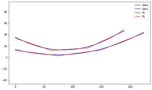
I made a Python notebook to separate the equations for each curve into 1000 discrete points. Then I ran a linear regression model to fit a curve of the points 1 - n, and a second curve of the n - 1000 points, looping from n = 2 to n = 999.
These results are from the combined output with the least squared error compared to the original.
Pictured is a plot showing the two sides of the curved bicone in red and blue, with the best fitting lines for each in black as well as a model in XF.
Results:
The antenna has a fitness score of 3.80627 with an error of 0.0759725.
This is much lower than the 5.71 of the curved antenna and 5.11 of the other attempt at straightening.
For the next attempt, we could consider constraining the endpoints to be the same as the original antenna to conserve the radius, and/or adding an extra line to fit the curve.
I've also attached a picture of what my notebook found for fitting 3 lines to the curve (not modeled or tested).
Professor Chen recommended using 3 sides and constraining the outer radii of the cones to match the original curved design.
Path to linear regression notebook: /users/PAS1960/dylanwells1629/developing/notebook.ipynb
Path to XF project: /users/PAS1960/dylanwells1629/straightened.xf |
| Attachment 1: output.png
|  |
| Attachment 2: image_(3).png
| .png) |
| Attachment 3: output.png
|  |
|
|
235
|
Wed Aug 2 00:17:32 2023 |
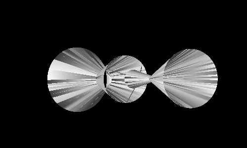
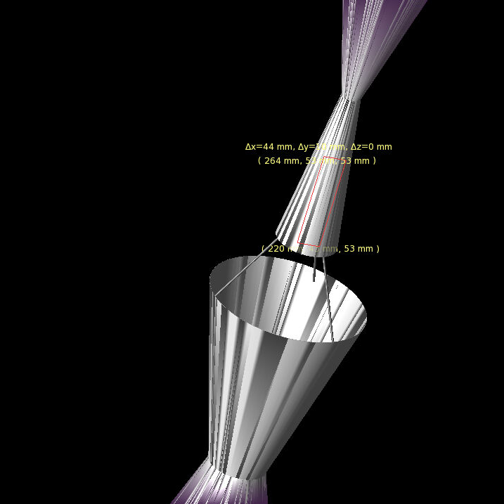
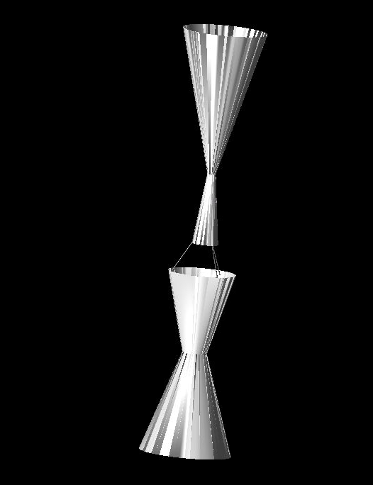
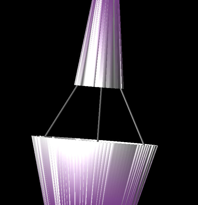
Jacob Weiler | XF Antenna Drawing Progress 08/02/2023 | I've been building in XF and have ran into some issues but currently have the following completed:
- Struts are placed, though they are not evenly spaced and the same. I have contacted XF to try and figure out how to get rotation/patterns to do what we need
- Circuit components and circuit board are in the xf file, though the components are not on the circuit board (I'm not totally sure how to put them on, that's the next step). The circuit components should be of spec, I looked up the part numbers from the previous ELOG post and grabbed the values from the manufacturer.
Here are the things that have not been completed/need answered:
- How to evenly space the struts connecting the shape (as stated previously, I've contacted XF to figure out how to do this easily. Im just bad at modeling in XF)
- Add circuit components to circuit board
- Add voltage and ground connections to the circuit board
- On the circuit diagram, figure out J1 and J2 connections. Meaning, which one connects to the signal from the cable and which connects to the other cone that is used as ground?
To see current antenna build go to: " /users/PAS1977/jacobweiler/GENETIS/XFzone/straightened_antenna_for_Jack.xf "
Attached are pictures in case there are issues pulling up model in XF. :)
|
| Attachment 1: sidepic.PNG
|  |
| Attachment 2: circuitboardplacement.PNG
|  |
| Attachment 3: fullpic.PNG
|  |
| Attachment 4: struts.PNG
|  |
|
|
234
|
Tue Jul 25 16:07:25 2023 |
Dylan Wells | Parallelizing XF and pueoSim in the loop | Standard Loop Architecture:
Complete an evolutionary step FOR EACH antenna before continuing on with the next step.
Steps:
1. Run the Genetic Algorithm for the entire population.
2. Run the XF radio simulation for the entire population.
3. Run the neutrino simulation software for the entire population.
4. Run root analysis and plots for the entire population.
However, due to constraints on the amount XF keys we have, we can only run 4-5 XF simulations at a time.
So, when the first antennas finish their XF simulations, their outputs will simply sit there until EVERY other antenna finished their XF simulations.
New Proposed Architecture:
Complete necessary evolutionary steps as a population, but string together those that don't rely on data from other antennas.
Steps:
1. Run the Genetic Algorithm for the entire population
2. Run the XF radio simulation for each antenna
- When an XF simulation finishes for an antenna, submit the pueoSim / root analysis jobs for that antenna
3. Run the plots for the entire population
This will allow us to complete most of our pueoSim computation while the XF portion of the loop is still running, cutting down the time between the final XF job finishing and the final pueoSim job finishing.
Test run of this new architecture with 100 antennas, 7,840,000 neutrinos per antenna.
| Part |
Time (seconds) |
| A |
1 |
| B1 |
1347 |
| Entire B2 |
54017 |
| B2 XF |
53063 |
| B2 remaining PUEO |
954 |
| E |
7 |
| F |
23 |
After the final XF job finished, the pueoSim simulations and analysis of outputted root files were completed in 954 seconds,
Comparison Between the Two Architectures (both using job optimization from Elog 232)
| Architecture |
Neutrinos |
Time In Loop (s) |
| Standard |
4,000,000 |
~6500 |
| New Proposed |
7,840,000 |
~950 |
Notes on Chart:
Source of data located in /users/PAS1960/dylanwells1629/buildingPueoSim/testingouts/times.txt and /fs/ess/PAS1960/HornEvolutionTestingOSC/GENETIS_PUEO/BiconeEvolution/current_antenna_evo_build/XF_Loop/Evolutionary_Loop/Run_Outputs/2023_07_24_test5/time.txt respectively)
Time from standard uses the time one of the 250 jobs running in parallel took in my testing of parallelizing processes inside of pueoSim jobs: 250 jobs * (40 * 40000 neutrinos per job) / 100 individuals = 4,000,000 neutrinos per individual)
The New Proposed time includes time spent analyzing the outputted root files to find fitness scores and errors, which would have taken around 100 seconds * population size for its number of neutrinos and files per individual (/fs/ess/PAS1960/HornEvolutionTestingOSC/GENETIS_PUEO/BiconeEvolution/current_antenna_evo_build/XF_Loop/Evolutionary_Loop/Run_Outputs/2023_07_23_test5/time.txt for data on this number)
So, this new architecture can provide more improvements for the amount and speed of neutrino simulation in the loop on top of the methods discussed in Elog 232.
This architecture could also be applied to see improvements in the Bicone and Hpol loops which are both affected by the limited number of XF keys.
Additional Notes:
1. For this new architecture test, each antenna uses 49 jobs for neutrino simulation instead of 2.5 previously. (49 pueoSim + 1 XF for 50 jobs per antenna, 5,000 jobs per generation)
2. The time for each antenna to submit, queue, and finish its neutrino simulation jobs must be less than the length of the XF job, or the extra time will accumulate for each antenna, losing much of the time benefits. (As long as it is less, the time spent on just pueoSim should be invariant under an increase in population)
3. The number of core hours spent on pueoSim jobs will be roughly the same for the same number of neutrinos as each job is shorter (except for a small contribution of the job overhead taking a higher percentage of total time for shorter jobs)
4. Initially I had thought that maybe queuing pueoSim jobs while running the XF jobs could slow down the queue for the XF jobs. So, I made the loop wait to submit the batch pueoSim jobs until we had space for all of them to be active with the ~250 max jobs per user.
Additionally, while observing my many tests, I didn't notice any correlation between the number of CPU peuoSim jobs in the queue and the number of GPU XF jobs out of the queue.
5. Branch I'm developing this on is here
6. The total time for the test generation was 15.4 hours, which is slightly longer than the ~14 hours from the 2023_05_08 run. However, this test also used double the population size, larger values for the range of antenna heights (on average about 3x taller), and 20x more neutrinos simulated per antenna. So, the actual speed is better than it first looks.
|
|
|
233
|
Mon Jul 24 15:51:28 2023 |
Ryan Debolt | Test Loop runs that need done. | |
Types of runs I need (May need some other people to help me run these):
-
Optimization runs
-
Non-error
-
Search over combinations of selection methods and genetic operators
-
Fix Sigma at 10%.
-
Do this for 10 runs for each
-
Re-run the best run for 100 tests to see if the results agree with 10 test results
-
This will be the main talking point
-
Save the plot for the best combination (proxy and metric)
-
Error
-
Re-run the best run for 100 tests with 3 different error amounts (0.1, 0.2, 0.3)
-
We will compare these results to the non-error run to talk about how errors may affect consistency/speed.
-
Save an example plot of an error test for each error (both metric and proxy score)
-
Population
-
Re-run the best run for 100 tests with 3 different population sizes (100, 500, 1000)
-
We will compare these results to the non-error run to talk about how population size affects consistency/speed.
-
Save an example plot of a population test for each size (just proxy score)
-
Demonstration runs (single runs, fitness score, no error population 100)
-
Crossover only
-
Mutation only
-
Reproduction only
-
Injection only
|
|
|
232
|
Tue Jul 18 22:04:22 2023 |
Dylan Wells | Parallelizing pueoSim jobs | Currently, the PUEO loop runs pueoSim with 1 pueoSim process per job submitted.
Each of these jobs has 1 node and 8 cores, however, pueoSim only needs a single core to run.
Here is some data I collected by running the same seed of pueoSim with different numbers of cores in the job:
| Processes |
Cores Per Job |
Run Time (1000 neutrinos) |
Neutrinos Per Second |
| 1 |
1 |
100 |
10 |
| 1 |
8 |
102 |
10 |
| 1 |
16 |
96 |
10 |
| 1 |
40 |
96 |
10 |
So, we should be able to run multiple processes of pueoSim without losing much performance.
Tests with more cores:
| Processes |
Cores per Job |
Run Time (1000 neutrinos) |
Neutrinos Per Second |
| 8 |
8 |
106 |
75 |
| 8 |
16 |
126 |
63 |
| 8 |
40 |
107 |
75 |
| 20 |
20 |
142 |
140 |
| 20 |
40 |
138 |
144 |
| 32 |
40 |
178 |
179 |
| 40 |
40 |
208 |
192 |
A test comparing the parallelization with the 40000 neutrinos per process we simulate in the loop:
| Processes |
Cores Per Job |
Run Time (40000 neutrinos) |
Neutrinos Per Second |
| 1 |
8 |
3226 |
12 |
| 40 |
40 |
6651 |
240 |
So, these tests suggest we can simulate neutrinos ~20 times faster than currently done in the loop by utilizing more cores per job.
This method of multiple processes per job should be applicable to how we run other simulation software like AraSim as well.
(Note: both of these jobs had comparable queue times of 27 and 31 seconds respectively.
Also, I have tested and seen that the outputted root files are identical for the same seed regardless of if ran with multiple processes at the same time or with processes in serial)
(data found in /users/PAS1960/dylanwells1629/buildingPueoSim/testingouts/times.txt)
How to run multiple processes of pueoSim:
Previous Call:
./pueoBuilder/build/components/pueoSim/simulatePueo -i pueo.conf -o ${PSIMDIR}/outputs/${gen}_outputs/$SLURM_ARRAY_TASK_ID -r $run_num -n $NNT -e $Exp > $TMPDIR/out.txt
Multiple Processes Test Call:
for ((i=0; i<$threads; i++))
do
./simulatePueo -i pueo.conf -o $TMPDIR -r $i -n $NNU -e 19 > pueo.out &
done
wait
Instead of just calling peuoSim once per job, we can use the & symbol and a loop to run $threads number of pueoSim processes in the background and then wait for them to finish. |
|
|
231
|
Wed Jul 12 21:30:56 2023 |
Alex Machtay | Zoom training on XF 07/12/23 | Recording of training on XFdtd by Alex Machtay on July 12, 2023.
https://osu.zoom.us/rec/share/FVKiTcQrRh8NLNYJADwugy0H2VjDo8ZlBsH16sJAGv2JINNwxxzyNfo5ueqVgOTO._XErF57Kz8KOM3a5
This link will expire in 120 days so note that we need to post a permanent recording.
Here's the GitHub repository with examples of Xmacros: https://github.com/Machtay/XFdtd_Scripts |
|
|
230
|
Thu Jul 6 14:52:09 2023 |
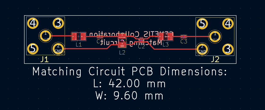
Jack Tillman | Building - Matching Circuit Schematic, PCB, and components | Attached are images of the matching circuit schematic and PCB design. A parts list is also attached in .pdf and .csv format. The .csv format can be imported into Digikey if necessary.
Table of component values:
| Inductors |
Capacitors |
SMA Connectors |
| 22 nH |
7.5 pF |
50 Ω |
| 27 nH |
5.7 pF |
50 Ω |
|
| Attachment 1: Matching_Circuit_Schematic.png
|  |
| Attachment 2: Matching_Circuit_PCB.png
|  |
| Attachment 3: Matching_Circuit_DigiKey_Cart.pdf
|
| Attachment 4: Matching_Circuit_DigiKey_Cart.csv
|
Index,Quantity,Part Number,Manufacturer Part Number,Description,Available,Backorder,Unit Price,Extended Price USD
1,3,WM26450-ND,733910083,"SMA RA JACK, PCB",3,0,5.1,15.3
2,4,490-GJM0335C1E7R5BB01DCT-ND,GJM0335C1E7R5BB01D,CAP CER 7.5PF 25V C0G/NP0 0201,4,0,0.1,0.4
3,2,490-17198-1-ND,GJM0335C1H5R7CB01D,CAP CER 5.7PF 50V C0G/NP0 0201,2,0,0.09,0.18
4,2,490-16032-1-ND,LQW2BAN27NJ00L,FIXED IND 27NH 2A 70 MOHM SMD,2,0,0.42,0.84
5,4,490-16028-1-ND,LQW2BAN22NJ00L,FIXED IND 22NH 1.9A 70 MOHM SMD,4,0,0.42,1.68
|
|
|
229
|
Thu Jul 6 13:12:04 2023 |
Jack Tillman | Straightened Sides AraSim Results | After discretizing and straightening the sides of the curved antenna that performed the best (Generation 13, individual 84) and running the antenna through AraSim, the following results and physics plots were generated. |
| Attachment 1: Straightened_Sides_AraSim_Results.pdf
|
| Attachment 2: Straightened_Sides_AraSim_Results.pptx
|
|
|
228
|
Thu Jun 29 12:05:45 2023 |
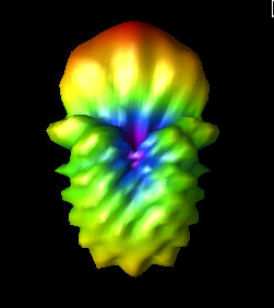
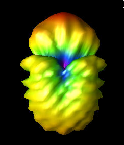
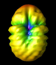
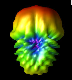
Alex M | Gain at various source heights | Here are a collection of antenna gain patterns with the antenna power source located at various heights at 500 MHz. The heights are indicated in the name of the images and were located at 3cm, 6cm, 12cm, and 24cm from the base. One thing to note is that the power source becomes longer as a function of height (since it's connected to the ridges, which slope back).
The 3D gain plots attached show the gain becoming more uniform until we get to the last one, where it seems to reinvert and be much stronger in the upward direction than below. I'll update this post with some polar slices for a more complete comparison between them.
EDIT: 07/17/23
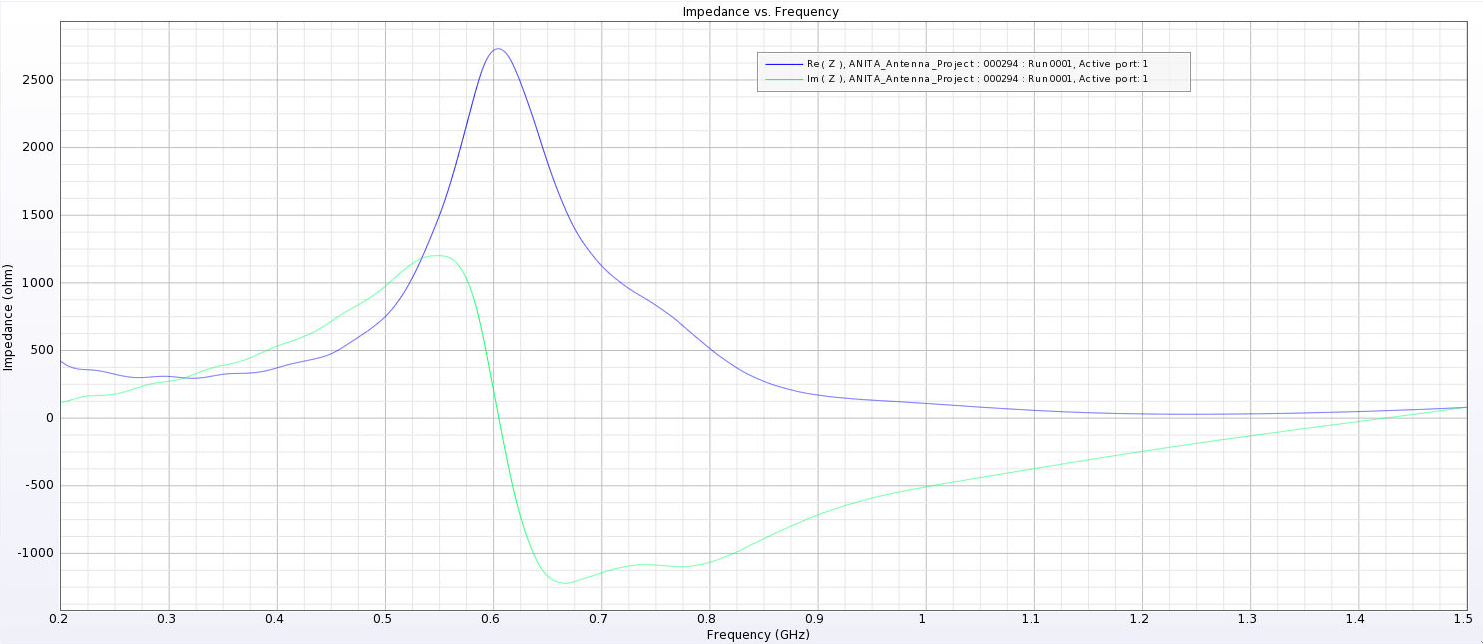
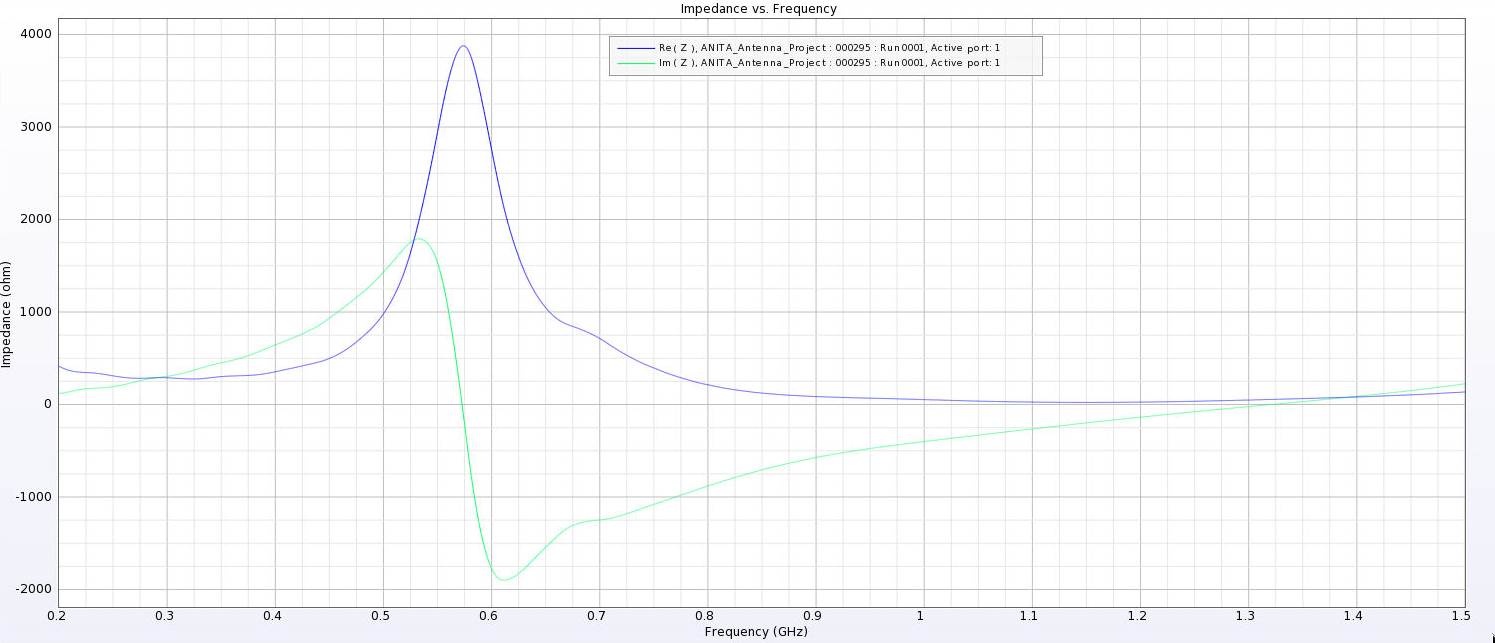
I've made a few adjustments and added plots of them.
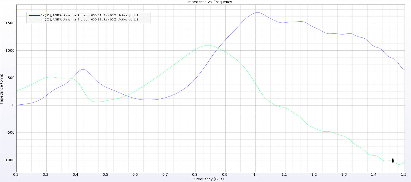
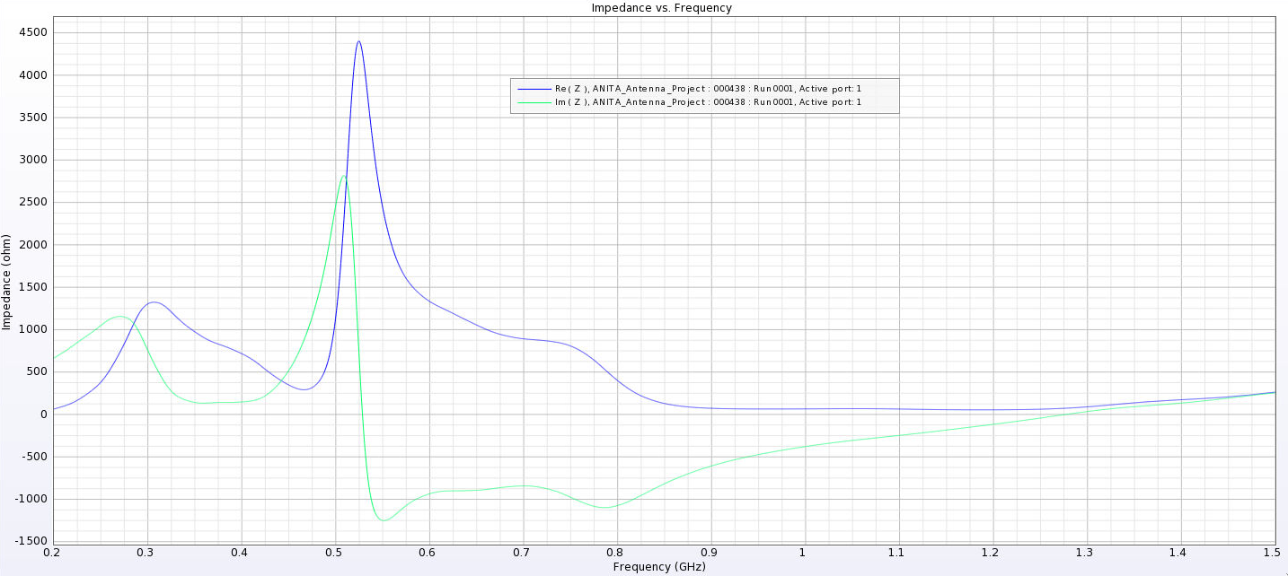
- First, I separated the ridges. Previously, the ridges touched at their inner corners. This electrically connected them and may be why we saw very high peaks in the first set of impedance plots. You can see the plots named Separated_Impedance_<x>_cm.png.
- This appears to have lowered the peaks considerably and also shifted them to lower frequencies. The peaks are still high when the source is placed high.
- We seem to be developing another peak at higher frequencies, although this also existed in the previous tests for the high sources.
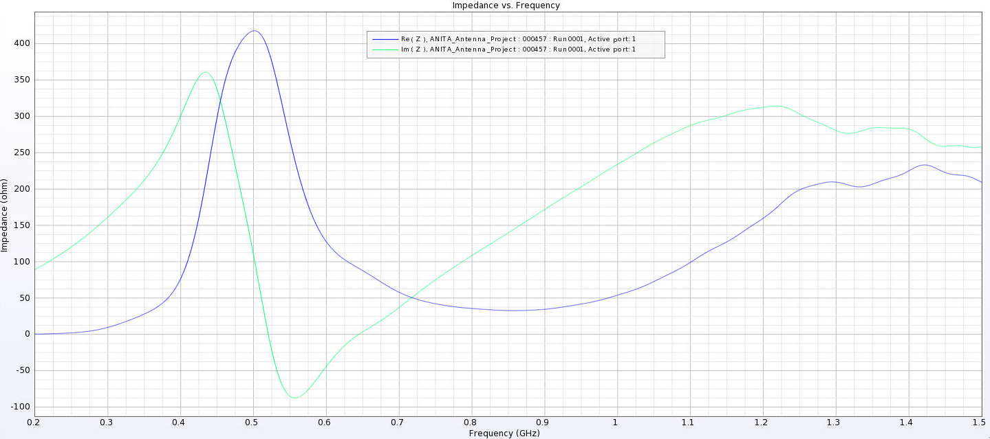
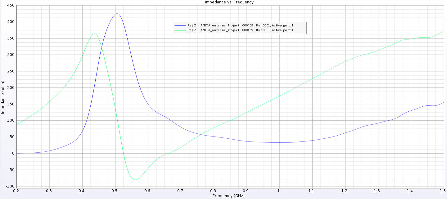
- After this, I added a waveguide and positioned the source between the extensions of the ridges into the waveguide. I've also added a picture that shows the waveguide in the geometry.
- The sources here are positioned from 1 cm below the ridges to 8 cm below the ridges. The naming convention is the same as above, except it includes "Waveguide" in the name.
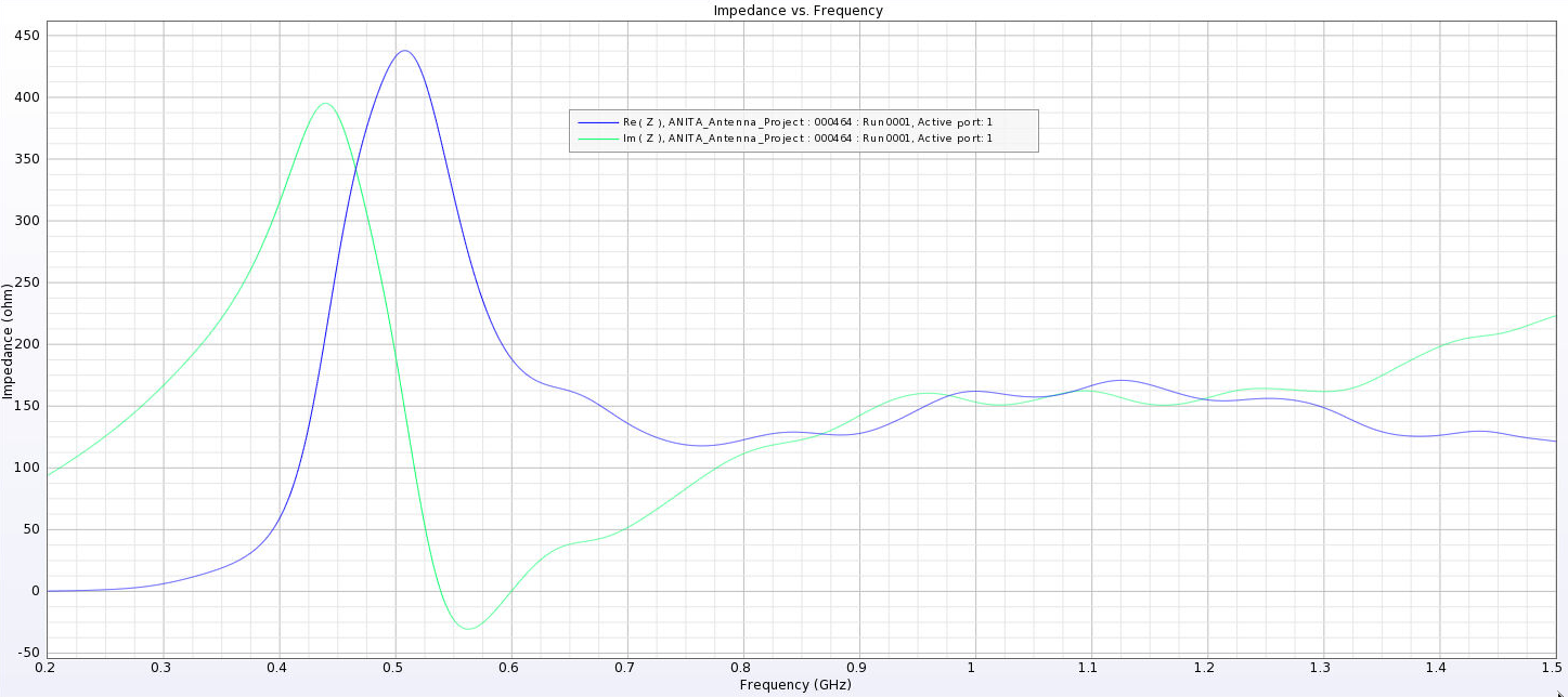
- The peaks are considerably lower here and seem consistent as we place sources further down. They are all below 500 Ohms, compared to as much as 4000 Ohms in the previous tests.
EDIT: 08/10/23
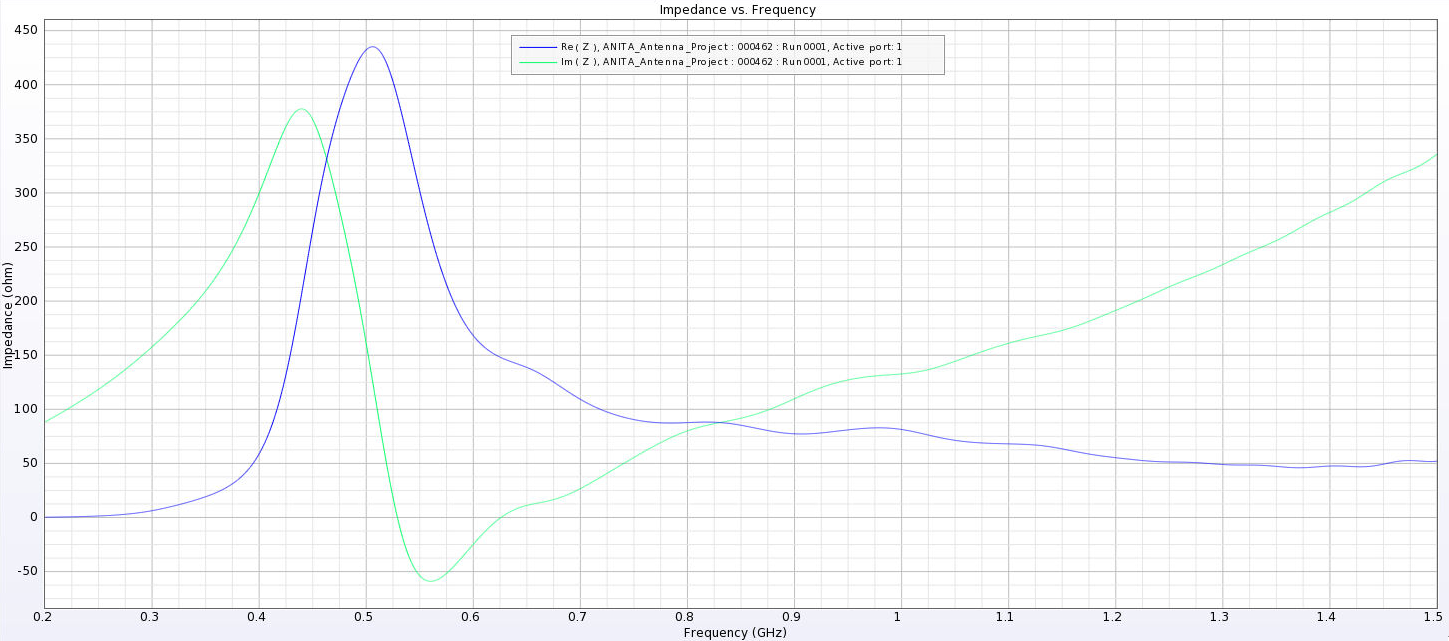
I've been trying more tweaks to the design to get rid of the peaks we see in the plots below. I'm having trouble actually getting the impedance to match close to the 50 Ohm value we expect from the cable. The best case situations seem to come from when the ridges are still touching, which we don't want. Here are the properties I've been changing:
- Ridge positions (gene in GA)
- We don't want the ridges to touch, but I can't get them to be very far from each other anyway. The minimum wavelength in our bandwidth would be 20 cm, but that's close to the size of the bottom of the antenna for when we make it large, so the separation is still small.
- When the ridges do touch is actually when I get the best matching,
- Bottom size (gene in GA)
- I've been changing the size of the bottom of the antenna. This is something that can change substantially between individuals in the GA, so even if I find a good value for this, the impedance it gives wouldn't be the same for all individuals we see in an evolution.
- This does seem to move the location of the impedance peak (in frequency) but I can't seem to get it fully out of band.
- Waveguide length
- I've been changing the length of the waveguide between 3 cm and 10 cm. We said that somewhere in the middle should be the most reasonable (the example antenna we saw looked to have a waveguide of ~5 cm long). It seems like the source position is more important.
- Source position
- I've been moving the position of the power source inside the waveguide. This seems to move around the peak and can lower its height, but I haven't been able to get peaks lower than ~400 Ohms, except in cases where the ridges are in contact.
I've added a picture of the best impedance I managed to get, but this involved an antenna with a small base and ridges touching. My next step is to just try a grid search by making many antennas automatically and simulating them all to look for any that have a nice impedance in our band. |
| Attachment 1: 3_cm.png
|  |
| Attachment 2: 6_cm.png
|  |
| Attachment 3: 12_cm.png
|  |
| Attachment 4: 24_cm.png
|  |
| Attachment 5: PUEO_Impedance_3_cm.png
|  |
| Attachment 6: PUEO_Impedance_6_cm.png
|  |
| Attachment 7: PUEO_Impedance_12_cm.png
|  |
| Attachment 8: PUEO_Impedance_24_cm.png
|  |
| Attachment 9: Separated_Impedance_3_cm.png
|  |
| Attachment 10: Separated_Impedance_6_cm.png
|  |
| Attachment 11: Separated_Impedance_12_cm.png
|  |
| Attachment 12: Separated_Impedance_24_cm.png
|  |
| Attachment 13: Separated_Waveguide_Impedance_1.png
|  |
| Attachment 14: Separated_Waveguide_Impedance_3.png
|  |
| Attachment 15: Separated_Waveguide_Impedance_6.png
|  |
| Attachment 16: Separated_Waveguide_Impedance_8.png
|  |
| Attachment 17: Best_Impedance_Plot_Horn_Antenna.png
|  |
|
|
227
|
Wed Jun 28 15:49:44 2023 |
Ryan Debolt | Optimization Runs 6/12/2023 | All data and plots discussed in this post are taken from this spreadsheet:
https://docs.google.com/spreadsheets/d/1BbpD81mugWQf10ozGDLI60takAn3tlvrq8ksT10yV5I/edit?usp=sharing
Run Details:
This optimization run was done to do a course search for the optimal set of parameters to run the GA with. This run used a fixed 100-individual population with a simulated error of 0.25 over 50 generations, to best replicate the current PUEO-loop environment. The selection methods have also been held fixed in this run. This run was tested using both the ARA and PUEO design to see if there were similarities in the best run type. This run encompassed 210 different run combinations that searched the following parameter space:
- 0-16 Reproduction, step sizes of 4
- 72-96 Crossover, step sizes of 4
- 4-16 Mutation, step sizes of 4
- 5-15 Sigma, step sizes of 5
Results:
Each run combination was run 10 times and we tracked the average number of generations it took for the distance metric to reach 0.05, which corresponds to a 0.95 true fitness score. The best runs for each design were as followed:
- ARA
- Parameters
- 12 Reproduction
- 72 Crossover
- 4 Mutation
- 5 Sigma
- Average gens to benchmark
- Standard Deviation
- PUEO
- Parameters
- 0 Reproduction
- 96 Crossover
- 4 Mutation
- 15 Sigma
- Average gens to benchmark
- Standard Deviation
We can see that these run types do not appear to have any strong correlations. In fact, looking at our complete data set, there does not appear to be a strong trend around any of the best runs. This issue became more prominent when we ran these best two run types for 100 tests rather than 10. When we did this, they returned averages of 44.4 generations for PUEO and 46.9 generations for ARA. For comparison, the average number of generations across all run types was 43.1 generations for PUEO and 42.8 generations for ARA. This seems to suggest that all of these run types are inherently inconsistent and regress to the mean given enough tests. Therefore, I do not believe we can draw any conclusions from this run.
Moving Forward:
Our ongoing hypothesis is that the size of the error could be causing inconsistency in how quickly our population can grow over time. Therefore, our next step is to repeat this experiment, but with zero error included, and see if we achieve results that show consistent behavior. If we can find more consistency in runs with no error, then we can more deeply explore the effects that error can have on GA growth. If there continues to be a lack of consistency, then we can look to other factors, such as population size, and try to find the root of the inconsistency.
|
|
|
226
|
Sun Jun 18 21:32:03 2023 |
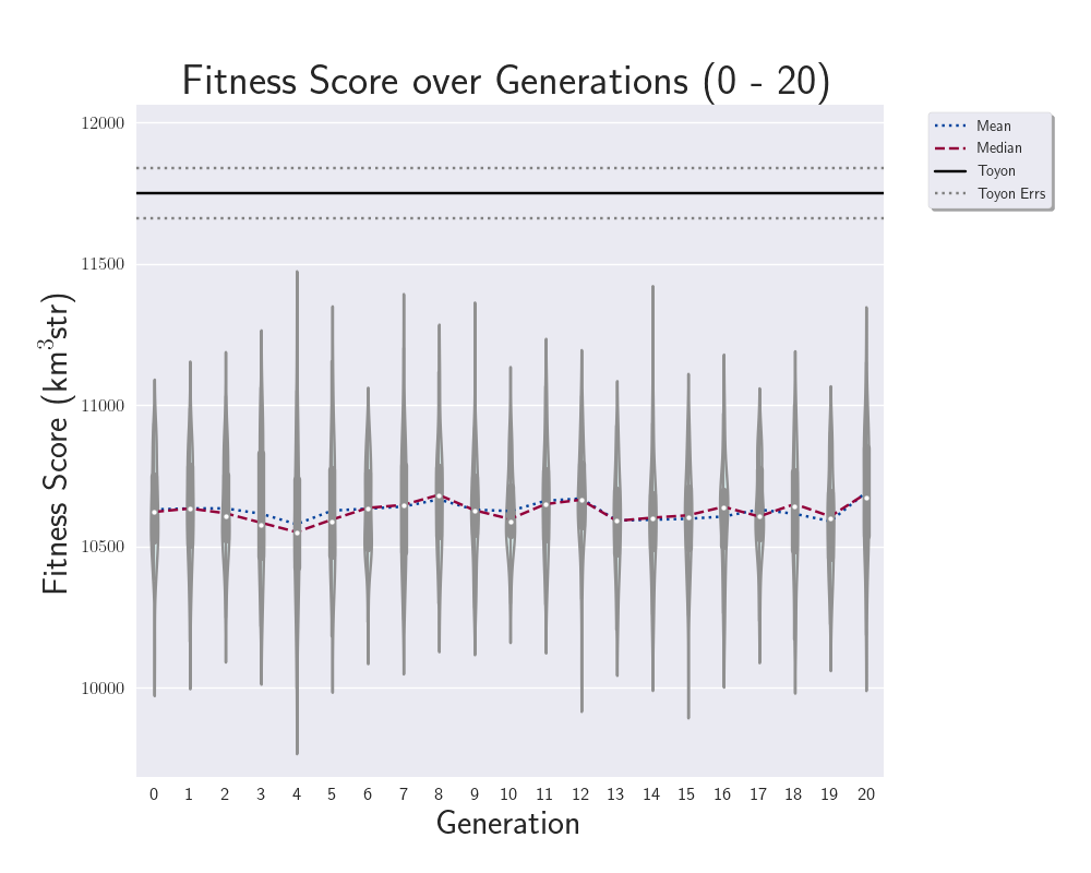
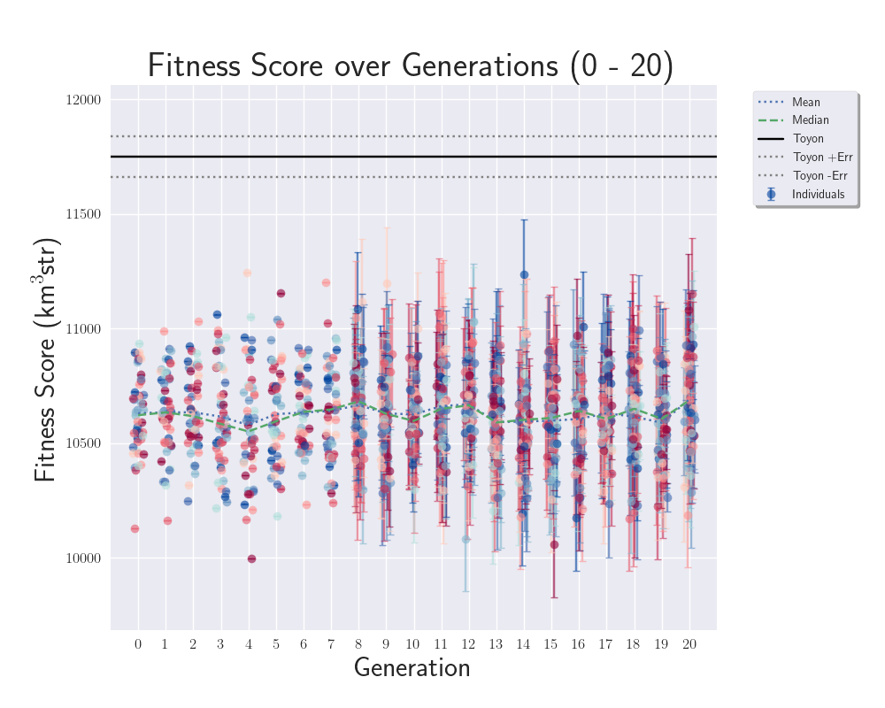
Dylan Wells | Default Toyon Antenna Simulation | To act as our comparison to the evolved antennas while plotting, we have done a simulation of pueoSim with 4,000,000 neutrinos for the measured toyon gains found in /fs/ess/PAS1960/buildingPueoSim/pueoBuilder/components/pueoSim/data/antennas/measured
In order to run the jobs, I used the runJobs.sh script found in /fs/ess/PAS1960/buildingPueoSim which submits job runs of 40,000 neutrinos at a time, mirroring what we do in the actual loop.
The resulting data is now located in /fs/ess/PAS1960/HornEvolutionOSC/GENETIS_PUEO/BiconeEvolution/current_antenna_evo_build/XF_Loop/Evolutionary_Loop/Toyon_Outputs
Veff: 11750.0503856
Plus Error: 89.0051458227
Minus Error:88.9007824246
The fitness score plots have been updated to read this value in as a comparison.
|
| Attachment 1: 248599981-8eacbc83-d42e-4da4-9746-bda05b2b4a38.png
|  |
| Attachment 2: 248599974-bee7a4db-34c6-4cfd-bde0-3682ff3ebaf7.png
|  |
|
|
225
|
Wed Jun 14 14:38:22 2023 |
Alex M | PUEO Antenna Dimensions | Here are my recommended starting genes for the initial generation of the upcoming run (confirmed that these will produce a working antenna in XF). We want to use the lowest values we can because we expect that a larger (namely, taller) antenna will perform better:
S, H, x0, y0, yf, zf, beta
7.50000,50.0000,1.0000,1.00000,1.00000,50.0000,0.2
- S: Half the side length of the bottom of the antenna
- H: height of the antenna
- x0: distance of the bottom of the ridge from origin
- y0: width of ridge at the bottom
- yf: width of ridge at top
- zf: final height of the ridge (cannot exceed H)
- beta: a curvature parameter for the ridges
|
|
|
224
|
Mon Jun 5 15:00:07 2023 |
Ryan Debolt | Github tests | We want to automate tests in pull requests in GitHub to run unit tests on individual functions to ensure they return the expected results. This will help prevent bugged code from being pushed to working branches. We will add a list of unit tests to this ELOG as we design them.
|
|